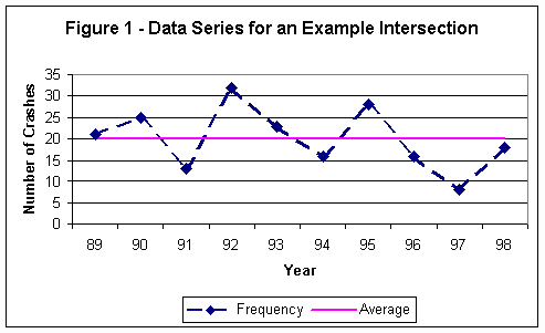
Perhaps the most important cause of erroneous conclusions in highway-related evaluations is the threat of regression to the mean. This threat is greatest when sites are chosen because of their extreme value in a given time period. When selecting high-hazard locations, for instance, the ones selected are those with the very worst recent crash record. It is generally true that the crash frequency or rate at a given location, all things remaining equal, will vary from year-to-year around a fairly consistent mean value The mean value represents a measure of safety at the location. The variations are usually due to the normal randomness of occurrence that is present. Because of that random variation, the extreme cases chosen in one period are very likely to experience lower crash frequencies in the next period. Simply stated, "the highest get lower and the lowest get higher."
Figure 1 is an example that demonstrates this. It shows the history of crashes at an intersection. This intersection might have been identified as a high-hazard location in 1993, based upon the rise in crashes in 1992.
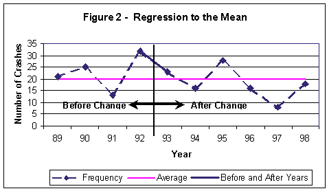
Even though a treatment may have been introduced early in 1993, any difference between the frequencies of crashes in 1992, and those in1993 and 1994 (See Figure 2) would, to some unknown degree, have to be attributed not to the treatment, but to the regression explanation. Thus, there would be a "threat to validity" of any conclusions drawn from a simple comparison of conditions before and after a change at a site.

In fact, should a decision be made not to make changes at the site (maybe due to lack of funds), the site would still be likely to show a reduction in crashes. Yet one would not be inclined to conclude that doing nothing, where a safety problem truly exists, is beneficial.

The issue of regression to the mean is only one of several present in a simple before-after comparison that will limit the ability to say how effective a particular program was, or will be. Most of the issues arise because the data from the before period is used as the clue as to what crash experience would be expected in the after period, had the program not been implemented. A simple before-after study assumes that the frequency used for the before period is the one to be expected in the after period. This assumption has several flaws, only one of which is the existence of regression to the mean.
Methods have been developed for eliminating or minimizing most of these problems. These may involve use of multiple-year data for the before and after periods, use of comparison groups, and application of the empirical Bayes approach. It is often wise to employ the services of a statistician in designing and implementing a program evaluation. The list of references, below, gives a few important resources.
References
Thomas D. Cook and Donald T. Campbell, Quasi-Experimentation, Rand McNally College Publishing Company, 1979
Council, et al, Accident Research Manual, FHWA Report DOT FH 11-9424, January 1980
Ezra Hauer, Observational Before-After Studies in Road Safety, Pergamon Press, 1997
William W. Wei, Time Series Analysis, Addison-Wesley Publishing Company, 1990