B
USEFUL TRANSFORMATIONS
Transformations are used to present data on a different scale. The nature of a transformation determines how the scale of the untransformed variable will be affected. In modeling and statistical applications, transformations are often used to improve the compatibility of the data with assumptions underlying a modeling process, to linearize the relation between two variables whose relationship is non-linear, or to modify the range of values of a variable. Transformations can be done to dependent variables, independent variables, or both.
References for Transformations
· Neter, John, Michael Kutner, Christopher Nachtsheim, and William Wasserman, and (1996). “Applied Linear Statistical Models”. 4th Edition. Irwin. Boston, MA.
· Myers, Raymond H. (1990). “Classical and Modern Regression with Applications”. 2nd Edition. Duxbury Press. Belmont, California.
· Glenberg, Arthur. M. (1996). “Learning From Data”, 2nd Edition. Lawrence Earlbaum Associates, Mahwah, New Jersey.
Although transformations can result in improvement of a specific modeling assumption, such as linearity or homoscedasticity, they can often result in the violation of others. Thus, transformations must be used in an iterative fashion, with continued checking of other modeling assumptions as transformations are made. It is possible that an improvement in one modeling assumption brought about by a transformation may result in a more serious violation of another assumption requisite to the model.
Another difficulty arises when the response or dependent variable Y is transformed. In these cases a model results that is a statistical expression of the dependent variable in a form that was not of primary interest in the initial investigation, such as the log of Y, the square root of Y, or the inverse of Y. When comparing statistical models, the comparisons should always be made on the original untransformed scale of Y. These comparisons extend to goodness of fit statistics and model validation exercises.
Transformations not only reflect assumptions about the underlying relation between variables, but also the underlying error structure of the model. For example, exponential transformations imply a multiplicative error structure of the underlying model, and not an additive error structure that is assumed in linear regression. For instance, when the underlying function Y = aexpbX + e is suspected, a log transformation will give ln(Y) = ln(aexpbX + e) = ln[(aexpbX )(1+ e/aexpbX)] = ln(a) + bX + ln(1+e/aexpbX)). Although the model is indeed linear, the error term is clearly not the one specified in ordinary least squares regression. In fact, the error term is a function of X, a, and b, and so is multiplicative. The upshot of this result is that error terms should always be checked after transformations are made to the model to make sure they are still compatible with modeling assumptions, which usually are normality and homoscedasticity (constant).
1) Transformations on a dependent variable will change the distribution of error terms in a model. Thus, incompatibility of model errors with an assumed distribution can sometimes be remedied with transformations of the dependent variable.
2) Non linearities between the dependent variable and an independent variable often can be linearized by transforming the independent variable. Transformations on an independent variable often do not change the distribution of error terms.
3) When a relationship between a dependent and independent variable requires extensive transformations to meet linearity and error distribution requirements, often there are alternative methods for estimating the parameters of the relation, namely, non-linear regression and generalized regression models.
4) Confidence intervals computed on transformed variables need to be computed by transforming back to the original units of interest.
5) Models can and should only be compared on the original units of the dependent variable, and not the transformed units. Thus prediction goodness of fit tests and similar should be calculated using the original units.
Taken in the context of modeling the relationship between a dependent variable Y and independent variable X, there are several motivations for transforming a variable or variables. It should be noted that many transformations are borne by the need to specify a relation between Y and X as linear, since linear relationships are generally easier to model than non-linear relationships. Thus, transformations done to Y and X in their originally measured units are merely done for convenience of the modeler, and not because of an underlying “problem” or “need” of the data themselves. Thus, transformations done to the dependent variable Y should be transformed back to the original units when a model is compared to other models, or when the model is presented to the professional community or to the general public. The general procedure for doing this is to linearize the relation between Y and X’s in the model, estimate model parameters, and then perform algebraic manipulations of the resulting equation to return Y to its original units.
The following figures show common transformations used to linearize a relationship between two random variables, X and Y. Provided is a plot of the relationship between X and Y in their untransformed states, and then some examples of transformations on X, Y, or both that can be used to linearize the relation.
Parabolic Transformations
Parabolic transformations are used to linearize a non-linear or curvilinear relation. The parabolic transformation is used when the true relation between Y and X is given as Y = a + bX + gX2. The transformation is done by simply adding a squared or quadratic term to the right hand side of the equation, which is really more than a mere transformation.
Of course the nature of the relationship depends on the values of alpha, beta, and gamma. Figure B-1a shows an example of a relation between Y and X when all parameters are positive, while Figure B-1b shows an example of the relation between Y and X when alpha and beta are positive and gamma is negative.
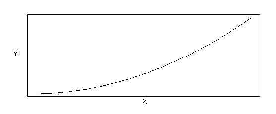
Figure B-1a Parabolic Relation (Functional Form: Y = a + bX + gX2 , where a > 0, b > 0, g > 0)
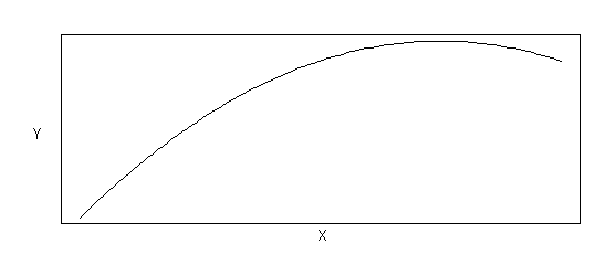
Figure B-1b Parabolic Relation (Functional Form: Y = a + bX + gX2 , where a > 0, b > 0, g < 0)
Hyperbolic Transformations
Hyperbolic transformations can be used to linearize a variety of curvilinear shapes. In essence, a hyperbolic transformation is used when the true relation between Y and X is given as Y = X/(a + bX), as shown in Figure B-2. By transforming both Y and X using the inverse transformation, one can generate a linear relationship such that 1/Y = b0+b1(1/X)+error. In this transformation, a = b1 and b = b0. Figure B-2a shows an example of a relation between Y and X when alpha is positive, while Figure B-2b shows an example of the relation between Y and X when alpha is negative.
Figure B-2a Hyperbolic Relation (Functional Form: Y = X /(a + bX), where a > 0)
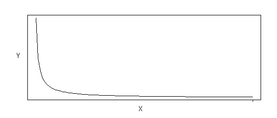
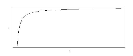
Figure B-2b Hyperbolic Relation (Functional Form: Y = X /(a + bX), where a < 0)
Exponential Functions
The natural log transformation is used to correct heterogeneous variance in some cases, and when the data exhibit curvature between Y and X of a certain type. Figures B-3a and B-3b show the nature of the relationship between Y and X for data that can be linearized using the log transformation. The nature of the underlying relation is Y = ae bx, where alpha and beta are parameters of the relation. To get this relation in linear model form, one transforms both sides of the equation to obtain ln(Y) = ln(ae bx ) = ln(a) + ln(e bx ) = ln(a) + bx = b0 + b1x. In linearized form b0 = ln(a) and b1 = b. Figure B-3a shows examples of the relation between Y and X for b > 0, while Figure B-3b shows examples of the relation between Y and X for b < 0.
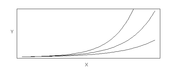
Figure B-3a Exponential Relation (Functional Form: Y = ae bX, where b> 0)
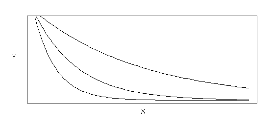
Figure B-3b Exponential Functions (Functional Form: Y = ae bX, where b< 0)
Inverse Exponential Functions
Sometimes the exponential portion of the mechanism is proportional to the inverse of X instead of untransformed X. The underlying relationship, which is fundamentally different than the Exponential relations shown in Figure B-3, is given by Y = aexpb/X. By taking the log of both sides of this relationship one gets the linear model form of the relation, ln(Y) = ln(a)+b/X = b0+1/Xb1. Figure B-4a shows examples of the inverse exponential relation when beta is positive, and Figure B-4b shows examples when beta is negative.
Figure B-4a Inverse Exponential Functions (Functional Form: Y = ae b / X,
where b> 0)
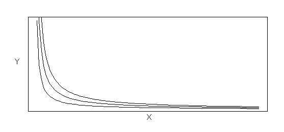
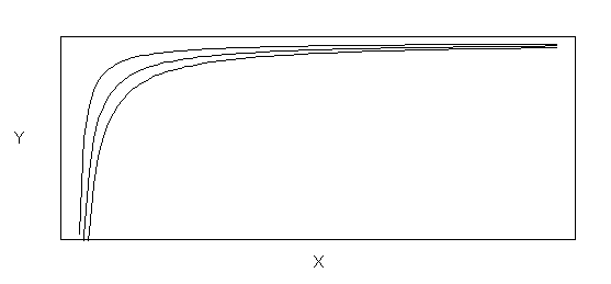
Figure B-4b Inverse Exponential Functions(Functional Form: Y = ae b / X,
where b< 0)
Power Functions
Power transformations are needed when the underlying structure is of the form Y = aXb, and transformations on both variables are needed to linearize the function. The linear form of the power function is ln(Y) = ln(aXb) = ln(a)+bln(X) = b0+b1ln(X). The shape of the power function depends on the sign and magnitude of beta. Figure B-5a depicts examples of power functions with beta greater than zero, while Figure B-5b depicts examples of power functions with beta less than zero.
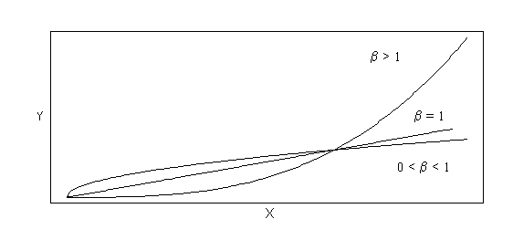
Figure B-5a Power Functions (Functional Form: Y = aXb, where b> 0)
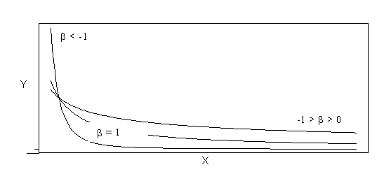
Figure B-5b Power Functions (Functional Form: Y = aXb, where b< 0)