^Chapter

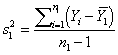
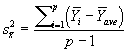
₄

Analysis of Variance is used to analyze the effects of one or more independent variables (factors) on the dependent variable. The dependent variable must be quantitative (continuous). The dependent variable(s) may be either quantitative or qualitative. Unlike regression analysis no assumptions are made about the relation between the independent variable and the dependent variable(s).  The theory behind ANOVA is that a change in the magnitude (factor level) of one or more of the independent variables or combination of independent variables (interactions) will influence the magnitude of the response, or dependent variable, and is indicative of differences in parent populations from which the samples were drawn.

Analysis is Variance is the basic analytical procedure used in the broad field of experimental designs, and can be used to test the difference in population means under a wide variety of experimental settings—ranging from fairly simple to extremely complex experiments. Thus, it is important to understand that the selection of an appropriate experimental design is the first step in an Analysis of Variance. The following section discusses some of the fundamental differences in basic experimental designs—with the intent merely to introduce the reader to some of the basic considerations and concepts involved with experimental designs. The references section points to some more detailed texts and references on the subject, and should be consulted for detailed treatment on both basic and advanced experimental designs.

1)       Single Factor Experiments: [The analyst wishes to quantify the effect of one factor with two or more levels (treatments) on the mean of a continuous response variable.]

·         Randomized Block Designs: [The effect of an unobserved “nuisance” variable is controlled by randomizing across “blocks”. Blocks are chosen because of a presumed unknown but potentially real effect on the response, and includes items such as test or manufacturing equipment, batches of raw materials, people, and time.]

·         Latin Square Designs: [Similar to the Randomized Block Design, but instead the analyst wishes to randomize the effect of two nuisance variables on the response instead of one.]

 

 

 

 

2)       Multiple Factor or Factorial Experiments: [The analyst wishes to quantify the effect of two or more factors with two or more levels (treatments) each on the mean of a continuous response variable.]

·         Two Factor Factorial Designs: [Factor A with a levels and Factor B with b levels are used to conduct replicate tests on each treatment combination, with a total of a x b treatment combinations, each with n replicates.]

·         2^K Factorial Designs: [There are a considerable number of cases where the factors each have only two levels. The number of treatment combinations when there are K factors is 2^K, thus an experiment with 3 factors, A, B, and C, each with two levels 1 and 0, results in 8 treatment combinations.]

3)       Multiple Factors Designs with Constraints—Fractional Factorial Designs: [In a study with many factors the researcher is primarily interested in the main and 2^nd order effects, and resource constraints often prohibit a full factorial design. For instance, in a 2⁶ factorial design, there are 64 runs required for one complete replicate. Of these 64 runs, only 6 are associated with main effects, and 15 are associated with 2^nd order interactions, thus some economy can be afforded by careful selection of a fractional factorial design.]

 

 

 

 

 

 

1)                   The mean of the dependent continuous variable Y varies as a function of the level(s) of factor(s) X for different populations.

2)                   The variance of Y for each population is the same.

3)                   The distribution of Y for each population is normally distributed.

Measurements on continuous variable Y

One or more explanatory or predictor variables X (Factors) that are either qualitative or quantitative having at least two or more levels (values)   

Estimated effect-size (difference in population means) between populations

Partitioning of sources of variation: random error and systematic error ‘caused’ by level of predictor variable(s)

F-ratio test statistic and associated probability

Interactions between variables that affect the population means

 

How is an analysis of variance model interpreted?

How is the F-test interpreted?

How are degrees of freedom interpreted?

What is an acceptable alpha level?
What is an acceptable beta level?

Should interaction terms be included in the model?

How many treatments should be included in the model?

How can randomization be accomplished?

What should be done when population variances are not equal?

What should be done when the populations are non-normal?
How does one know if the errors are normally distributed?
What should be done to cope with unequal sample sizes?

What will confounded variables do to model results?

 

Pavements

Waheed, Uddin, Alvin H. Meyer, and W. Ronald Hudson. (1984). Study Of Factors Influencing Deflections Of Continuously Reinforced-Concrete Pavements. Transportation Research Record #993 pp. 47-54. National Academy of Sciences.

Adel W. Sadek, Thomas E. Freeman, and Michael J. Demetsky. (1996). Deterioration Prediction Modeling of Virginia's Interstate Highway System. Transportation Research Record #1524 pp. 118-129 National Academy of Sciences.

Bridges

Mitsuru, Saito, Kumares C. Sinha, and Virgil L. Anderson (1995). Bridge Replacement Cost Analysis. Transportation Research Record #1490 pp. 23-31. National Academy of Sciences.

Fugler, Mark D., R. Richard Avent, and Mohamed Alawady. (1995). Systematic Evaluation of Structural Deterioration in Underwater Bridge Substructures. Transportation Research Record #1476 pp. 139-146. National Academy of Sciences.

Traffic

Graham, Jerry L., Douglas W. Harwood, and Michael C. Sharp. (1979). Effects of Taper Length on Traffic Operations in Construction Zones. Transportation Research Record #703 pp. 19-24. National Academy of Sciences.

Humphreys, Jack B., Donald J. Wheeler, Paul C. Box, and T. Darcy Sullivan. (1979). Safety Considerations in the Use of On-Street Parking. Transportation Research Record #722 pp. 26-35. National Academy of Sciences.

Safety

Hadi, Mohammed A., Aruldhas Jacob, Chow Lee-Fang and Wattlewort Joseph A. (1995). Estimating Safety Effects of Cross-Section Design for Various Highway types Using Negative Binomial Regression. Transportation Research Record #1500 pp. 169-177. National Academy of Sciences.

 

Lyles, Richard W. (1980). Evaluation of Signs for Hazardous Rural Intersections. Transportation Research Record #782 pp. 22-30. National Academy of Sciences.

 

Bergan, A. T., L. G. Watson, and D. E. Rivett. (1980). Mandatory Safety-Belt Law: The Saskatchewan Experience. Transportation Research Record #782 pp. 16-21. National Academy of Sciences.

Planning

Prothero, Jon C. and Thomas A. Seals. Evaluation of Educational Treatment for Rehabilitation of Problem Drivers. Transportation Research Record #672 pp. 58-63. National Academy of Sciences.

 

Martha S. Lester, James W. Dare, and William T. Roach. (1979). Technique for Monitoring Automobile Occupancy: Research in the Seattle Area. Transportation Research Record #701 pp. 7-15. National Academy of Sciences.

Materials

Benson, Paul E. (1995). Comparison of End Result and Method Specifications for Managing Quality.

Transportation Research Record #1491 pp. 3-10. National Academy of Sciences.

 

Freund, Rudolf J. and William J. Wilson (1997). “Statistical Methods”. Revised Edition. Academic Press. Boston, MA.

Glenberg, Arthur. M. (1996). “Learning From Data”, 2^nd Edition. Lawrence Earlbaum Associates, Mahwah, New Jersey.

Johnson, Richard A. (1994). “Miller & Freund’s Probability & Statistics for Engineers”. 5^th Edition. Prentice Hall. Englewood Cliffs, New Jersey.

Montgomery, Douglas C. (1991). “Design and Analysis of Experiments” 3^rd Edition. John Wiley & Sons. New York

Neter, John, Michael Kutner, Christopher Nachtsheim, and  William Wasserman, and (1996). “Applied Linear Statistical Models”. 4^th  Edition. Irwin. Boston, MA.

Postulate effects of levels of categorical X on continuous response variable Y based on theoretical or past empirical research

Underlying theory should motivate the development of an analysis of variance model whenever possible. Simplified, a relation is thought to exist such that the level of a factor variable is thought to affect the mean of a dependent variable Y. Theories and empirical evidence should suggest which factor levels of the independent variable are important, and how they are thought to affect Y.

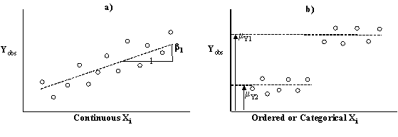
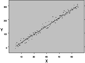
Figure 1 shows two possible relationships between a response variable Y_obs and an independent variable X_i. Figure 1a shows a regression model used when both variables X and Y are continuous. Figure 1b shows the results of an ANOVA when the response variable Y is continuous and the X variable (Factor) is at two levels (in figure 1b the observations are scattered across X so they can be seen, for a true categorical response with two levels the observations would fall on two vertical lines). The X variable may be either qualitative or quantitative.

 

Figure 1: Typical Regression (a) and ANOVA (b) Relationships Between Response Variable Y_obs and Independent Variable X_i

 

 

 

 

 

 

 

ANOVA is used to determine the effect of two or more levels of one or more factors on the mean response of the independent variable. Although the mean response of the independent variable may change with factor/level combinations, an assumption in ANOVA is that the variance of the independent variable is constant at all factor/level combinations. 

Collect data through experimentation or observation

Data would be collected in decreasing preference through experimentation, quasi experimentation, or observation (see Chapter 1). Recall that causality can be ascertained through experimentation only, and that quasi-experiments and observational studies suffer increasingly from lack of control of potentially influential variables, rendering conclusions from them less certain.

A sampling plan should be devised (see Chapter 1) to collect data sufficient for detecting statistically significant differences between the groups of observations in the ANOVA. Recall from Chapter 1 that sample sizes are determined by drawing a pilot sample, computing variances, estimating the anticipated effect size between groups of observations, and then back calculating from the ANOVA formula to obtain the necessary sample sizes n for each of the groups. Balanced designs lead to the simplest computations in ANOVA models; thus, sample sizes for each group of observations should be equal whenever possible.  As models become more complex sample size calculations also become more complex. Fortunately, numerous software packages are available for helping the analyst estimate sample size requirements for simple and some more advanced ANOVA designs.

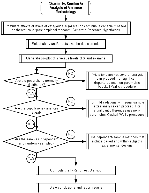
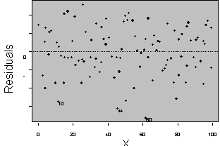
Generate Boxplot of Y versus levels of X and examine

The boxplot is useful for visualizing the magnitudes of effects of various levels of a factor X on the response variable Y. It is analogous to the scatter plot used in linear regression to examine the relation between an independent variable X and the dependent variable Y. Figure 2 shows a typical boxplot for three levels of a factor variable X and a response variable Y. The solid white horizontal stripe in the middle of each box represents the median of Y for each of the three factor levels of X. The height of the box represents the difference between the 25^th and 75^th percentiles of Y for each of the factor levels of X. A median that is in the center of the box suggests a symmetric distribution or spread of the data around the mean. The top and bottom end bars show the 5^th and 95^th percentiles of Y with respect to each of the factor levels respectively. Again, equal distances of the bars from the box represent symmetry in the distribution. Recall that for a normal distribution the mean and median are equivalent, and the distribution is symmetric.

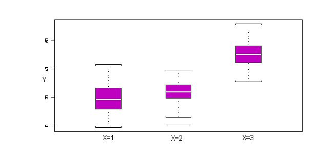Figure 2: Example Boxplot of Y Versus 3 Factor Levels of X

 

 

 

 

 

 

 

 

 

The boxplot is used to assess normality of Y with respect to the factor levels of X, and to assess the effect size. The effect size is the effect that the level of X has on the mean of Y, and is estimated by the difference between the means of the samples for different factor levels of X. In the figure, for example, it can be seen that the mean of Y for X=1 is approximately 20, while the mean of Y for X=2 is approximately 25. The mean of Y for X=3 is approximately 50. The analytical task of the ANOVA approach is to determine if the difference in the means between two factor levels, say X=1 and X=2, is a result that would arise by reasonable chance (high likelihood), or if the observed difference is rather supported by a low-likelihood event, giving evidence that a causal agent brought about the observed difference.

The boxplot provides a visual inspection of the effect sizes for various factor levels, and allows the symmetry of the distributions at various factor levels to be inspected, one of the assumptions of the ANOVA methodology.

Are ANOVA assumptions met: normally distributed Y; equal population variances; independently sampled populations?

As in all statistical models, the ANOVA model has assumptions that should be thought of as requirements. When requisite assumptions are not met, in most cases a work-around analytical solution is available. The difficult part, most often, is determining when to use a work-around solution and when the ANOVA is appropriate. This section provides guidance on how to determine the appropriateness of the ANOVA assumptions, and what to do if the assumptions are not met.

Is Y Normally distributed?

The ANOVA model assumes that all populations (at each level of X) are approximately normally distributed. There are several plots and tests that can be used to assess normality, including the Q-Q plot, the boxplot, and the non-parametric chi-square test of distributions (see Chapter 6), and the Kolmogorov-Smirnoff test. The statistical tests underlying the ANOVA methodology are robust, and so moderate departures from normality can be ignored (Glenberg, 1996). For severe departures from normality, a Kruskal-Wallis H test procedure should be used to compare sample means. Because the Kruskal-Wallis H test is not as powerful as ANOVA, it should only be used when the requisite ANOVA assumptions are not met.

Are the population variances equal?

All of the population variances are assumed to be equal in the standard ANOVA framework. Called the “homogeneity of variance” assumption, mild departures from this assumption can be tolerated without compromising the validity of the method. For moderate to severe departures from this assumption, however, the non-parametric Kruskal-Wallis H test should be used.

A common sampling distribution used to test whether variances were drawn from the same normal population (or two populations with the same variance s²) is the F. If S₁ and S₂ are the sample variances of independent random samples of size n₁ and n₂ respectively, then the sampling distribution of the test statistic F is approximately F distributed with n₁ (numerator) and n₂ (denominator) degrees of freedom such that:

 

Large values of the F statistic lead to a rejection of the “homogeneity of variance” null hypothesis. Note that the analyst can let S₁² be the larger of the two sample variances in the computation of the F statistic. Small values of the F statistic tend to support the alternative hypothesis that the sample variances are “equivalent”, and that observed differences reflect natural variability inherent in two samples drawn from a single population with variance s².

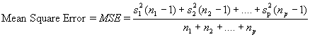
For cases with more than two factor levels and subsequently more than two variances to test, one needs to consider additional tests. One such test is Bartlett’s test (see Montgomery, D.C., 1991, pp. 102). Other tests include Hartley and modified Levene tests for homogeneity of variance (see Neter et al., pp. 763). The Hartley test is now briefly discussed.

The Hartley test is used to assess the homogeneity of variance assumption in ANOVA. It is fairly sensitive with respect to the normality assumption, and so the distributions should be fairly normal. In addition, it requires equal sample sizes in order to be conducted. For a more robust test with respect to normality and for a test that does not require equal sample sizes, apply the modified Levine test (Neter et al., 1996, pp. 763). The Hartley test statistic is simply the ratio, denoted H, of the largest sample variance to the smallest sample variance. Values of H near 1 support the null hypothesis—that all variances are approximately equal. Large value of H supports the alternative hypothesis—that not all variances are equal. One must consult statistical tables (see Neter et al.) to determine the probabilities associated with various values of H, given the number of independent populations r and common degrees of freedom df.

 

 

Were the Populations Sampled Independently?

The assumption underlying the data for ANOVA is that samples are independently sampled. In other words, entities representing one factor level do not affect the probability of entities being selected at another level. A violation of this assumption would occur, say, if two household members were selected in a study, one for each of two samples. Thus, a sampling unit or entity would be in one sample only if another member of the household was in the other sample. There are methods developed for dependent samples, and these include paired comparisons, paired data, and random assignment methods used in ANOVA. For detail on these advanced applications of ANOVA see Glenberg (1996), Freund and Wilson (1997), Montgomery (1991), or Neter et al. (1996).

Select alpha and/or beta and the decision rule

Recall that the alpha level is the probability of committing a type I error, while the beta level is the probability of committing a type II error (see Chapter 1). A type I error is made when the analyst incorrectly rejects the null hypothesis—that the sample means of Y are significantly different at various levels of factor X. A type II error, in contrast, is made when the analyst incorrectly fails to reject the null hypothesis when in fact it is false. Recall that type I and type II error rates are related (see Chapter 1), and selection of smaller type I error rate leads to a larger type II error rate.

The determination of which statistical error is less desirable depends on the research question and consequences of the two error types. Both types of error are undesirable, and thus attention to proper experimental design prior to collection of data will help the engineer minimize the probability of making errors.

Often the probability of making a type I error, alpha, is set at 0.05 or 0.10 (5% and 10% error rates respectively). The selection of alpha often dictates the level of beta for a given hypothesis test. The computation of beta under different hypothesis testing scenarios is beyond the scope of this chapter, and the reader is referred to more complete references on the subject such as Glenberg (1996).

There is nothing magical about a 5% alpha level. Selection of an appropriate alpha level should be based on the consequences of making a type I error. For instance, if human lives are at stake when an error is made (which can occur in accident investigations, etc.), then an alpha of 0.01 or 0.005 may by appropriate. On the other hand, if the result merely determines where monies are spent for improvements (e.g. congestion relief, transit level of service improvements, etc.), then perhaps a less stringent alpha is most appropriate. Finally, the consequences of types I and II errors need to be considered together, as they are not independent.

Compute the F-ratio test statistic (Using the formulas appropriate for the specific experimental design)

The analyst has selected the appropriate experimental design, and has collected data by applying this design. After all standard assumptions of ANOVA have been met; one can proceed with the analytical computations involved with ANOVA—typically conducted by using packaged software programs. The null hypothesis in the ANOVA framework is typically given by; H₀: m₁ = m₂ =…..= m_p, and the alternative hypothesis is that the null hypothesis is incorrect, and that the means of the population samples at various factor levels of X are different.

The F statistic is central to the ANOVA framework, and is used to test the null hypothesis. The following formula for the F statistic is used to test the equality of p sample means: where;
  
 

 
 
 

p = number of population samples (1 for each factor level of X)

N = total sample size, n₁ + n₂ +….+ n_p

The F statistic is based on the following general principal. Two estimates of the sample variance are obtained, MST and MSE. If the null hypothesis is true, and the sample means are equivalent, these two independent estimates of the sample variance will be approximately equivalent, and their ratio will be approximately equal to 1. When the null hypothesis is not true, MST will overestimate the sample variance, and the F ratio will become large. As F and MST become increasingly large, one begins to suspect that the null hypothesis is not true. Note that the F ratio does not provide evidence as to which sample mean is different than the rest, only whether the estimate of error obtained through the computation of MST gives evidence that all sample means are not equivalent.

Draw conclusions and report results

In an analysis of variance the investigator is trying to determine whether an observed difference in population means is other than would occur by mere chance alone. Stated another way, the analyst is trying to determine whether there is evidence to suggest that there is a systematic effect of the treatment(s) (difference(s) between the two populations), and what this effect is. The F-ratio test is used to determine the probability that the data would have been observed assuming the null-hypothesis is true—that population means are equal. An F value with an associated probability lower than the alpha level suggests that data observed under the null hypothesis are unlikely to have occurred by chance according to some decision criteria set by the analyst. High probabilities associated with an F-value suggest that random sampling differences alone could have produced the observed data. It should be noted that alpha is arbitrarily chosen by the analyst, and the decision to accept or reject a chance explanation of the data is a function of the level of risk acceptable to the analyst.

Designed experiments, where the treatment is the only difference between the populations, are best suited for analysis of variance. In designed experiments random effects from ‘nuisance’ factors are randomized so that they contribute to the error term in way that enables it to be distinguished from the systematic or treatment effect. In addition, other factors thought to affect the response are held constant from trial to trial. The control of these nuisance factors, the available resources, and the number of factors and their levels help the analyst to select the appropriate experimental design for the research problem. Additional information on experimental designs can be found in Neter et al., 1991, and Montgomery, 1991.

In many transportation applications, research investigations cannot be carried out as a designed experiment, and thus are more ‘observational’ in nature. Inferences made from observational studies are much more difficult, because confounded variables and other systematic biases can enter the data in unknown ways.

From the example it can be seen that the statistical results of an analysis of variance do not provide definitive conclusions as to the underlying processes—they merely provide clues to support or refute an engineering claim. It should be stressed that no amount of statistics can replace logic and critical thinking about a process; however, they can and should be used to inform a process and lend insights that lead to theory refinement, further testing, further theory refinement, etc. In any experiment or observational study, there should be sufficient a priori reason to believe that an underlying material process would affect the results. In the signing example, an engineer should believe a priori that the new sign would affect motorist’s speeding behavior differently than the existing sign. Lack of a material explanation for observing the results is grounds to refute the results of even the most convincing statistical outcome.

 

How is an analysis of variance model interpreted?

The standard one-way ANOVA model is given by:

                

where;

Y_ij = value of the response variable in the j^th trial for the i^th factor level or treatment,

m_i = model parameters, population mean for i^th factor level or treatment,

e_ij = normally and identically distributed error terms with mean 0 and variance s²,

i = 1,….,r, where r is the number of factor levels or treatment groups,

j = 1,…,n_i, where n_i is the number of cases for the i^th factor level or treatment.

The parameters m of the ANOVA model are estimates of the factor level or treatment means, while the error term e is an estimate of the spread of the data around treatment means. Thus, an observation is merely the sum of the factor level or treatment mean and an error term. In general, the more different are the factor level means compared to the error terms, the more statistically defensible is the model.

How is the F-test interpreted?

The F-ratio test in ANOVA is the ratio of MST (mean square treatment) to MSE (mean square error). Under the null hypothesis, that is when the null hypothesis is true and factor level means are equal, the F-ratio follows the F distribution. Values of F near unity support the null hypothesis, and suggest that there is insufficient evidence to support different means for factor level populations. Large values of F support the alternative hypothesis, and suggest that factor level or treatment means are different.

Specifically, the F test is interpreted in the following manner. The F ratio statistic provides the long-run probability that the observed data would have occurred given the null hypothesis.

How are degrees of freedom interpreted?

Degrees of freedom are associated with sample size. Every time a statistical parameter is estimated on a sample of data the ability to compute additional parameters decreases. Degrees of freedom are the number of independent data points used to estimate a particular parameter. With regard to analysis of variance, there are p - 1 independent data points to estimate treatment means, and N – p data points available to estimate the error variance.

What is an acceptable alpha level?

The alpha level, or type I error rate, is the level or risk associated with making a type I error. It is determined by the analyst a priori, and is based upon an assessment of risk acceptable for rejecting the null hypothesis (population means are different) when in fact it is true.

What is an acceptable beta level?

The beta level, or type II error rate, is the level or risk associated with making a type II error. It is determined by the analyst a priori, and is based upon an assessment of risk acceptable for failing to reject the null hypothesis (population means are different) when in fact it is false. Of course, the analyst begins by determining what magnitude of effect is desired to be detected. Large effects requires smaller samples, while smaller effects require larger samples, all else being equal.

Operational Characteristic Curves are plots of the type II error probability of a statistical test for a particular sample size versus a parameter that reflects the extent to which the null hypothesis is false. The curves are used by the analyst to determine an appropriate number of replicates so the experiment will produce results that are sensitive to potentially important differences in treatments (factor levels).

Statistical software is becoming improved with regard to assessing beta, and recent and future advances will enable the analyst to avoid the use of Operational Characteristic Curves. These curves are explained and tabulated in Montgomery, 1991, and power analysis tables can be found in Neter, et al., 1996.

Several general observations can be made about the relationship between sample size, power, alpha, beta, and the sample variance:

1.       The larger is alpha, the smaller is beta. In other words, for a given sample size, sample variance, and difference in population means, an increase in alpha (willingness to commit a type I error) results in a reduction in beta (willingness to commit a type II error).

2.       The larger is the effect size delta, the smaller is beta. Thus, for a given alpha level, sample variance, and sample size, larger effects (differences between population means) will reduce beta.

3.       Smaller sample variances for a given sample size, effect size, and alpha will reduce beta. Thus, reducing sample variance either through more precise measurements or increased sample size will reduce beta, all else being equal.

Should interaction terms be included in the model?

Suppose, that the effect of factor level X₁ on Y depended not only on the factor level X₁, but also on the factor level X₂. The variables X₁ and X₂ are called main effects. A multiplicative effect is called an interaction between factor levels X₁ and X₂. An interaction between two variables is called a second-order interaction, between three variables is called a third-order interaction, etc. In general main-effects are more important than interactions, and the higher the order of interaction, the less influential the effect is on Y. Identifying interactions in some cases is a main objective of ANOVA.

Interactions in ANOVA occur when two treatments or factor levels are thought to affect the mean of the population differently than the additive effects of the two treatments.

How many treatments should be included in the model?

The objective of most modeling efforts is to economize the model. In other words, the analyst generally wishes to explain as much of the data complexity with as few variables as practicable. It is generally better to favor a simpler model to a more complex one, simply because interpretation and implementation are simplified also. On the other hand, if the phenomenon is sufficiently complex, then making too simple a model may sacrifice too much explanatory or predictive power. In the ANOVA context, many models are built upon experimental data, and often the effect of one or several factors is being isolated from other potentially important factors. In observational contexts, the analyst should be careful to identify and isolate the main effects to be studies, and then randomize to the extent possible other ‘nuisance’ factors.

How can randomization be accomplished?

Randomization or random assignment is different than random sampling. Random sampling is the task undertaken to obtain a sample that is representative of the population being studied. Random sampling is necessary to make inferences about the population being studied.

Random assignment can be used to make inferences about the independent variable when a random sample cannot be obtained (it can also be used with random samples). Random assignment occurs when subjects are assigned to treatments in a random fashion. In this way, systematic effects that might confound the results would be randomized across treatment groups. When random assignment is performed, the effect of the independent variable is separated from other potentially confounding effects. 

What should be done when population variances are not equal?

Called “homogeneity of variance”, the assumption of equal variances is important in the computation of the pooled estimate of variance in the ANOVA methodology. When population sample sizes are equal, mild violations of this assumption are acceptable. When there is evidence that population variances are very different, then a non-parametric Kruskal-Wallis test should be used.

What should be done when the populations are non-normal?

The statistical tests underlying the ANOVA methodology are robust, and so moderate departures from normality can be ignored (Glenberg,1996). For severe departures from normality, a Kruskal-Wallis H test procedure should be used to compare sample means. Because the Kruskal-Wallis H test is not as powerful as ANOVA, it should only be used when the requisite ANOVA assumptions are not met.

How does one know if the errors are normally distributed?

There are several methods to assess normality of a distribution. Graphical methods involved visual assessment of a distribution, and involve histograms, boxplots, and normal or Q-Q plots. For normal distributions several noteworthy characteristics make visual inspection fairly straightforward:

1.       A normal distribution is symmetric, or bell-shaped.

2.       The mean and median are the same in a normal distribution, thus the ‘middle most’ value should correspond with the average value.

More formal methods involve comparing an observed distribution to a hypothesized distribution using a chi-square test or similar. This non-parametric test is used to assess the statistical evidence of observing distributions as dis-similar given natural sampling variability.

What should be done to cope with unequal sample sizes?

Unequal population sample sizes in ANOVA are analyzed using unbalanced designs methods. Essentially these are methods that correct the computations needed to handle the unbalanced designs. For guidance on unbalanced designs and other more complicated designs consult some of the ANOVA references listed in this section.

What will confounded variables do to model results?

Confounding of variables is likely to occur only when observational studies are conducted and randomization cannot be performed. Confounding is essentially a missing variable(s) problem. When a variable or factor that is partly responsible for producing data, but it is omitted from the analysis, then the effect-sizes in the ANOVA model are biased.

 

The direction of omitted variable bias depends on the relation between the included and omitted variables. For positively correlated omitted variables the model parameters are biased high (in absolute magnitude), while for negatively correlated omitted variables the model parameters are biased low (in absolute magntitude).

 

Linear regression is used to model a linear relationship between a continuous dependent variable Y and one or more independent variables X. Most applications of regression aim to identify what variables are associated with Y, to postulate what causes Y, to predict future observations of Y, or to assess control over a process or system (quality control). Generally, explanatory or ‘causal’ models are based on data obtained from well-controlled experiments (e.g. conducted in laboratory), predictive models are typically based on data obtained from observational studies, and quality control models, although seldom appropriate for regression models, are based on data obtained from a process or system being controlled or monitored.

 

1)                   The dependent variable Y varies linearly with the independent variable(s) or X’s.

2)                   The observations on dependent variable Y are assumed to have been randomly sampled from the population of interest.

3)                   Y is caused by or associated with the X’s, and the X’s are determined by influences (variables) ‘outside’ of the model and are measured without error.

4)                   There is uncertainty in the linear relation between Y and the X’s, as reflected by a scattering of observations around the ‘curve’ of a hypothesized relationship (known as residuals or error term).

5)                   The distribution of the error terms must be identified to result in an efficient and unbiased model.

6)                   The independent variables or “X’s” are measured without error.

In many practical cases some of the assumptions of the ordinary least squares (OLS) regression model are not satisfied. In addition, some difficulties with making the OLS framework fit to specific problems can be solved by using simpler methods. Listed below are some special situations that arise in regression modeling, requiring specialized regression techniques to be applied in order to solve them. In many cases an OLS violation can be determined by inspecting graphs (1 and 2) or computing simple diagnostic measures (3). In other cases (4 and 5), the analyst must scrutinize the selected variables and hypothesized relationships to identify a potential violation. The interested reader should refer to the Linear Regression References for detailed discussion and applications of these methods. Listed below are some of the common OLS regression violations and their commonly applied solutions:

1)                   Non-normality of error terms. In OLS linear regression the response variable is assumed to be normally distributed. If departures from normality are serious, then making inferences about the true population parameters may be quite incorrect. There are several possible corrective actions to be taken. First, transformations may be applied to the response to obtain a normally distributed variable. Second, if the response follows a known statistical distribution, identified a priori or empirically, such as the Poisson, Negative Binomial, Logistic, etc., then a generalized regression model may be fitted to the data. Finally, Monte Carlo and bootstrapping techniques might be applied to determine with confidence the sampling distributions of the estimated model parameters. For references on these topics consult Greene, 1990, Neter et al., 1996, and Myers, 1990.

2)                   Non-linear relation between Y and X’s. There are some cases when a non-linear relationship between Y (dependent) and the X’s (independent) variables can be successfully linearized within the OLS linear regression framework using transformations (see technical details in this chapter and the Appendix). However, caution must be exercised because many transformations also affect the error term, which may render other OLS requirements invalid. In cases where model parameters are inherently non-linear and all linear regression requirements cannot be met with transformations or when the modeler desires to estimate non-linear model parameters directly, non-linear regression models should be applied. For references see Neter, et al. 1996, and Myers, 1990, and Glossary of Highway Quality Assurance Terms,” Transportation Research Circular Number E-C010, July 1999.

3)                   Non-constant variance. When the error term exhibits non-constant variance, the OLS framework is inappropriate. Techniques such as weighted least squares, ridge regression, and generalized regression techniques may be appropriate when the error terms are heteroscedastic, or non-constant. For references see Neter et al. 1990 and 1996, Myers, 1990, and Greene, 1990.

4)                   Errors are correlated across time. When the error terms are correlated across time they are said to be autocorrelated. Autocorrelation typically occurs in situations where sampling units (e.g. people) are recorded at regular time intervals, making them correlated across time. Time series methods are appropriate when errors are correlated across time. For references see Greene, 1990, and Neter et al., 1996.

5)                   Random error in the independent variables. Although the dependent variable is assumed to be measured with error, it is assumed that independent variables are measured with negligible error. There are numerous “fixes” for dealing with poorly measured independent variables, including instrumental variables techniques, method of proxy variables, and structural equations models. For references see Greene, 1990, Neter et al., 1996, and Myers, 1990, or Weed & Barros, “Demonstration of Regression Analysis with Error in the Independent Variable,” Transportation Research Record 1111, 1987, pages 48-54.

6)                   One or more independent variables is influenced by Y or by another X.  It is assumed that Y is influenced by the X’s, and not in the reverse direction. When the value of Y influences the value of one or more of the X’s, the affected X’s are said to be endogenous. Simultaneous equations models and in some cases structural equations models can be used to deal with these situations. For references see Greene, 1990 and Kline, 1998.

Continuous variable Y

One or more continuous and/or discrete variables X

Functional form of relation between Y and X’s.

Strength of association between Y and X’s (individual and collective).

Proportion of uncertainty explained by hypothesized relation. 

Confidence in predictions of future/other observations on Y given X.

 

 

 

 

 

 

 

Pavements

Sallack, David J. and Stephen M. Greecher. (1979). Evaluation of Highway Maintenance Cost and Organization in Pennsylvania. Transportation Research Record #727 pp. 17-24. National Academy of Sciences.

Darter, Michael I. (1980). Requirements for Reliable Predictive Pavement Models. Transportation Research Record #766 pp. 25-31. National Academy of Sciences.

Al-Suleiman, Turki I., Kumares C. Sinha and Virgil L. Anderson (1988). Effect of Routine Maintenance on Pavement Roughness. Transportation Research Record #1205 pp. 20-28. National Academy of Sciences.

Materials

Kandhal, Prithivi S., Foo Kee Y., D'Angelo and John A. (1996). Control of Volumetric Properties of Hot-Mix Asphalt by Field Management. Transportation Research Record #1543 pp. 125-131. National Academy of Sciences.

Stroup-Gardiner, Mary and David Newcomb. (1988). Statistical Evaluation of Nuclear Density Gauges Under Field Conditions. Transportation Research Record #1178 pp. 38-46. National Academy of Sciences.

Shah, Alam and Dallas N. Little. (1985). Evaluation of Fly Ash and Lime-Fly Test Sites Using a Simplified Elastic Theory Model and Dynaflect Measurements. Transportation Research Record #1031 pp. 17-27. National Academy of Sciences.

Singh, Gurdev and Shafiq Khalil Hamdani. (1980). Characterization of Bitumen-Treated Sand for Desert Road Construction. Transportation Research Record #766 pp. 31-42. National Academy of Sciences.

Bridges

Fitch, Michael G., Weyers Richard E., and Johnson Steven D. (1995). Determination of End of Functional Service Life for Concrete Bridge Decks. Transportation Research Record #1490 pp. 60-66. National Academy of Sciences.

Traffic

Stokes, Robert W., Vergil G. Stover and Carroll J. Messer. (1986). Use and Effectiveness of Simple Linear Regression to Estimate Saturation Flows at Signalized Intersections. Transportation Research Record #1091 pp. 95-101. National Academy of Sciences.

Hall, Fred L. and Denna Barrow. (1988). Effect of Weather on the Relationship Between Flow and Occupancy on Freeways. Transportation Research Record #1194 pp. 55-63. National Academy of Sciences.

Persaud, Bhagwant and Leszek Dzbik. (1993). Accident Prediction Models for Freeways. Transportation Research Record #1401 pp. 55-60. National Academy of Sciences.

Safety

Jovanis, Paul P. and Hsin-Li Chang. (1986). Modeling the relationship of Accidents to Miles Traveled. Transportation Research Record #1068 pp. 42-51. National Academy of Sciences.

Squires, Christopher A. and Peter S. Parsonson. (1989). Accident Comparison of Raised Median and Two-Way Left-Turn Lane Median Treatments. Transportation Research Record #1239 pp. 30-40. National Academy of Sciences.

Salman, Nabeel K. and Kholoud J. Al-Maita. (1995). Safety Evaluation at Three-Leg, Unsignalized Intersections by Traffic Conflict Technique. Transportation Research Record #1485 pp. 177-185. National Academy of Sciences.

Environment

Clemena, Gerardo G. (1981). Empirical Relationship Between Mesoscale Carbon Monoxide Concentrations and Areal Vehicular Emission Rates. Transportation Research Record #789 pp. 5-14. National Academy of Sciences.

Cohen, Stephen L. and Gary Euler. (1978). Signal Cycle Length and Fuel Consumption and Emissions. Transportation Research Record #667 pp. 41-48. National Academy of Sciences.

Dabberdt, Walter F. and Howard A. Jongedyk. (1978). Atmospheric and Wind Tunnel Studies of Air Pollution Dispersion Near Highways. Transportation Research Record #670 pp. 43-55. National Academy of Sciences.

Planning

Moon, Henry E., Jr. (1988). Stepwise Regression Model of Development at Nonmetropolitan Interchanges. Transportation Research Record #1167 pp. 46-50. National Academy of Sciences.

Hendrickson, Chris and Sue McNeil. (1984). Estimation of Origin-Destination Matrices with Constrained Regression. Transportation Research Record #976 pp. 25-32. National Academy of Sciences.

How is a regression equation interpreted?

How do continuous and indicator variables differ?

How are partial slope coefficients interpreted?

How is the F-test interpreted?

How are t-statistics interpreted?

How are r and R² interpreted?

How are confidence intervals interpreted?

How are prediction intervals interpreted?

How are degrees of freedom interpreted?

What are standardized regression coefficients?

Should interaction terms be included in the model?

How many variables should be included in the model?

What methods can be used to linearize the regression relation?

What methods are available for fixing heteroscedastic errors?

What methods are used for fixing serially correlated errors?

What methods are used for fixing correlated errors?

What can be done to deal with multi-collinearity?

What is endogeneity and how can it be fixed?

How does one know if the errors are normally distributed?

What if the errors are not normally distributed?

Freund, Rudolf J. and William J. Wilson (1997). “Statistical Methods”. Revised Edition. Academic Press. Boston, MA.

 

Glenberg, Arthur. M. (1996). “Learning From Data”, 2nd Edition. Lawrence Earlbaum Associates, Mahwah, New Jersey.

 

Kline, Rex B. (1998). Principles and Practice of Structural Equation Modeling. The Guilford Press. New York.

 

Greene, William, (1990).  Econometric Analysis.  Macmillan Publishing Company.

 

Johnson, Richard A. (1994). “Miller & Freund’s Probability & Statistics for Engineers”. 5th Edition. Prentice Hall. Englewood Cliffs, New Jersey.

 

Myers, Raymond H. (1990). “Classical and Modern Regression with Applications”. 2nd Edition. Duxbury Press. Belmont, California.

 

Neter, John, William Wasserman, and Michael Kutner  (1990). “Applied Linear Statistical Models”. 3rd Edition. Irwin. Boston, MA.

 

Neter, John, Michael Kutner, Christopher Nachtsheim, and William Wasserman, and (1996). “Applied Linear Statistical Models”. 4th Edition. Irwin. Boston, MA.

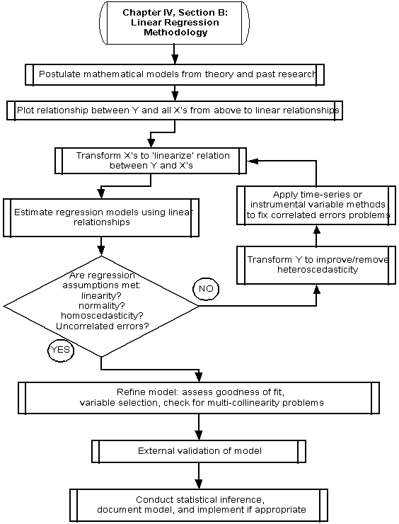
Postulate mathematical models from theory and past research.

Underlying theory should motivate the development of a regression model whenever possible. Theories that describe the nature of the relationship between variables often provide insight as to initial or starter model specifications for the regression model.

 

Past empirical or experimental research on the phenomenon under study is an additional source for postulating relationships between variables to be employed in a regression model. That is, past models estimated on similar data will reveal logical starting points for estimating regression models in the conduct of new or continuing research. Past research should reveal the nature of linear relationships between variables, distributional properties of the model error terms, and the magnitude and sign of estimated model coefficients.

 

In regression methodology it is assumed a priori that a linear relationships exists in the population of interest between a response or dependent variable Y, and explanatory or independent variables X₁, X₂, ….., X_P such that:

                

where;

Y_i is the value of the response variable in the i^th trial,

b₁, b_2,… b_P-1   are the partial effects of explanatory variables X₁, X₂, ….., X_P on Y,

b₀ is the Y intercept, or point at which the regression model crosses the Y-axis,

X₁, X₂, ….., X_P are known constants (resulting primarily from experimental research) or random variables (resulting primarily from observational research), and

P is the number of parameters in the model,

e_i is the error term expressing the difference between the regression equation and observations,

e_i is a random error term with mean E [e_i] = 0,and variance VAR [e_i]=s², and

e_i and e_j are uncorrelated so that the covariance COV [e_i e_j] = 0 for all i, j:  i ¹ j, i = 1, .., n.

 

It is presumed in statistical theory that the model for the population of interest is never known or knowable. Instead, the population model is estimated using a random sample of data drawn from the population. The sample data are then used to estimate the model:

                 

where;

b _1, b ₂,…, b _P-1 are the estimated partial effects of explanatory variables X₁, X₂, .., X_P on Y, and

e_i is the estimated error term expressing the difference between the regression equation and observations.

 

Each sample drawn from the universe will result in different values of betas due to natural sampling variability. Thus, a regression line based on a sample of observations is not likely to fall directly on the regression line of the population of interest. Several aspects of sampling variability with respect to regression models should be noted:

1)       The regression line for the population of interest is never known, and is estimated by estimating a regression model on a sample of data.

2)       Random sampling is relied upon to ensure that the sample possesses similar qualities and characteristics to that of the universe.

3)       A sample-based regression line that is ‘numerically close’ to the universe regression line is preferred to one that is ‘numerically distant’. In other words, small sampling variability of the betas is desirable—and are said to be more efficient.

4)       It is desirable that the long-run average of betas (obtained by estimating a large number of models based on different random samples) be equal to the associated universe parameters. An estimated parameter (beta) with this property is said to be unbiased.

 

Plot Relationship Between Y and All X’s to Identify Linear Relations.

Recall that the assumed relationship between the dependent variable Y and the independent variables (X’s) is linear. In other words, linear regression is limited to models where the presumed effect of X is constant over the range of Y. This is not as restrictive as it may first appear, since transformations of the X’s, Y, or both, can often linearize the relation between Y and X such that linearity between them is obtained. It is cautioned, however, that use of transformations can in some cases cause other problems in the regression that offset the advantages of the transformations (see Are Regression Assumptions Met?). Past research should also help to illuminate linear relationships between the variables under study.

Transform X’s to Linearize Relation Between Y and X’s

Appendix B provides an extensive list of transformations that can be used to linearize a relationship between two variables. It should be noted, however, that use of transformations to improve linearity can invalidate the assumption of constancy of the error terms (homoscedasticity), and so transformations cannot be used without consequence. In addition, transformations of the dependent variable, Y, can result in non-intuitive expressions of the phenomenon under study, and so comparisons of alternative models should always be done using the original un-transformed units of Y.

Estimation of Regression Models

Because the values of the true beta coefficients for the model based on the entire population of interest is not known or knowable, they must be estimated using data obtained from a random sample. Because the betas estimated from a sample will vary from sample to sample, the estimated betas are random variables. In linear regression the standard method for estimating model parameters is the method of ordinary least squares.

Method of Ordinary Least Squares (OLS)

The OLS estimators of the betas for a linear regression model are unbiased and have minimum variance of all competing unbiased estimators. In the OLS method of finding estimators, the sum of the n squared deviations of Y_i from their expected values is minimized. In other words, the method of OLS minimizes the difference between the observed Y’s and the Y’s predicted by the regression model.

To illustrate, consider a regression model with one predictor variable, X₁. Using the method of OLS, the estimators of b₀ and b₁ are those values of b₀ and b₁ that minimize Q for a given random sample of observations, where;

The values of b₀ and b₁ that minimize Q can be derived by obtaining the partial derivatives of Q with respect to b₀ and b₁. The partial derivatives can then be set to zero and solved for the betas (b₀ and b₁). Computing second partial derivatives can be checked for positive values, indicating minimum values of the function Q. For regression models with more than two parameters to be estimated, matrix algebra is used to solve for the regression parameters.

Properties of the fitted regression model

Once an estimate of the theoretical universe model has been estimated from a random sample of data drawn from the population of interest, the fitted regression model is obtained. The fitted regression model possesses some interesting and sometimes useful properties:

1)       The expected value of Y is equal to the population regression function:  E [Y] = b₀ + b₁X₁.

2)      The sum of the squared residuals is a minimum:
                  3)       The sum of residuals is zero:
 

4)      The sum of observed values equals the sum of fitted values, therefore the means are also equal:

5)     The sum of the weighted residuals is zero when the residual in the i^th observation is weighted by the independent variable in the i^th observation.

6)       The sum of the weighted residuals is zero when the residual in the i^th observation is weighted by the fitted value for the i^th observation.

7)      The regression line always goes through the point X_ave, Y_ave.

The Estimated Error Terms Variance s²

 

The sum of squared errors, or sum of squared vertical deviations of the fitted values from observed values is given by:

                                                              

 

The sum of square errors, SSE, has N - P degrees of freedom associated with it, where P is the number of parameters estimated in the regression model. The mean deviation from the regression function of individuals observations, or MSE, is given by:

                 

where N is the sample size and P is the number of estimated parameters in the regression model.

Using ordinary least squares estimation, MSE is an unbiased estimator of s² for the regression model.  An estimator of the standard deviation is simply the square root of MSE.

 

Using Indicator, or Qualitative Independent Variables in the regression model

Thus far, regression modeling has been presented with the assumption that the independent variables are continuous variables, for example household income, moisture content, elapsed time, material stress, length, etc.  Often, however, an analyst is interested in the effect of qualitative variables such as gender, type of composite, type of fracture, etc. An analyst can include nominal and ordinal variables into the regression model. Discrete variables are modeled differently than continuous variables in a regression model.  The use of indicator variables is best illustrated by example.

 

Suppose the analyst estimates a regression model using three indicator variables representing 3 out of 4 levels of a categorical variable, denoted by X₂ through X₄ for levels 2 through 4 respectively. Assume that X₁ is a continuous variable in the model (unrelated to the indicator variables). The following estimated regression function would be obtained (the subscript i denoting observations is dropped from the equation for convenience):

           

Careful inspection of the model shows that for any given observation, at most one of the new indicator variables can remain in the model. This is a result of the 0-1 coding, when X₂ = 1,  X₃ and X₄ are equal to 0 by definition. Thus, the regression model becomes four different models based on which indicator variable is equal to 1:

 

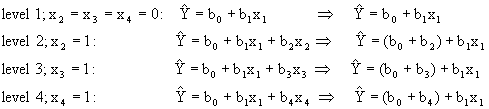
Inspection of these regression models reveals an interesting result. First, depending on which of the indicator variables is coded as 1, the slope of the regression line with respect to X₁ remains fixed, while the y-intercept coefficient changes by the amount of the coefficient of the indicator variable. Stated more simply, indicator variables, when entered into the regression model in this form, make adjustments to the y-intercept term only:

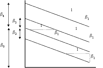
Graphically, the model is shown in Figure 3. It shows that the slope of X₁ is the same for any value of the indicator variable, however, the y-intercept changes by the estimate of betas associated with the level of the indicator variable.

Figure 3: Graph of Regression Lines with Three Levels of Indicator Variables Used to Adjust Y-Intercept

 

 

 

 

 

 

Suppose the analyst suspects that each indicator variable interacts with income differently. That is, each level of licensed driver responds has a unique relationship with household income. Interacting indicator variables with one or more continuous variables will afford this flexibility in the regression. To include these interactions in the model, the former model can be revised to obtain:

 

The difference between this regression model and the model shown previously is that each indicator is entered in the model twice: as a stand-alone variable and interacted with the continuous variable X₁. This more complex model can be reduced to the following set of regression equations again depending upon the level of the indicator variable.  

 

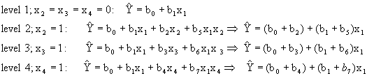
The interpretation of these coefficients is considerably different than before. Each level of the indicator variable is now free to have an effect on both the y-intercept and slope of the regression function with respect to the variable income. Graphically, the model now looks like the regression equations in Figure 4.

Figure 4: Graph of Regression Lines with Six Levels of Indicator Variables Used to Adjust Y-Intercept and Partial Slope Coefficients

 

 

 

 

 

 

 

 

 

 

 

 

 

 

 

 

 

 

 

 

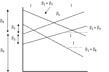
The figure shows that the regression model is really four different regression functions, of which both the slope and the y-intercept depend on the level of the indicator variable. 

Interactions on Continuous Variables

Often times there is a relationship between one or more independent variables that is worthy of inclusion into the regression function.  To illustrate, consider the two estimated regression functions:

 

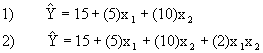
Regression function (1) is a function with two variables, X₁ and X₂, while regression function (2) contains an interaction term, X₁X₂.  In equation 1, no matter the level of X₁, an estimate for Y is obtained by adding 15 + 10X₂.  Conversely, no matter the level of X₂, one can simply add 15 + 5X1 to obtain an estimate for Y.  In other words,  X₁ and X₂ act independently of each other with regard to their effect on Y.

Equation 2 is different.  It contains an interaction term, which accounts for the fact that X₁ and X₂ do not act independently.  The function says that the relationship between X₁ and Y is dependent upon the value of X₂, and conversely, that the relation between X₂ and Y is dependent upon the value of X₁.  The nature of the dependency is captured in the interaction term, X₁X₂.

Essentially, the equation with the interaction term can be re-arranged to obtain:

It can be seen that the resulting change in Y given unit change in one of the independent variables (while the other is held constant) depends on the level of the level of the interacted variable.  Note that this is different than before, because the change in Y per unit change in X stayed constant across all levels of X. There are numerous cases when the effect of one variable on Y depends on the variable of another independent variable, and in these cases interactions should be incorporated into the regression model.

Are the regression model assumptions met?

Estimation of regression models is an iterative process. Once regression parameters have been estimated, functional forms have been specified, and indicator variables and interaction terms have been added to the model, it is wise to check the original assumptions, or requirements, of the regression equation. Not checking assumptions of the regression is poor practice, and may result in dissemination of a poor model. Thus, checking the assumptions is of utmost importance and should be the standard procedure in regression modeling.   

There are at least nine situations in which the conditions for a regression equation are not ideal:

1)       Non-linearity of the regression function,

2)       Heteroscedasticity of the error terms,

3)       Lack of independence of the error terms,

4)       Extreme influence by outlying observations,

5)       Non-normality of error terms,

6)       Omission of important variables from the regression model,

7)       Multi-collinearity of independent variables,

8)       Poorly measured X variables, and

9)       Endogeneity.

Each of these departures from the regression assumptions is now discussed.  Note that both graphical and quantitative methods are used to assess departures from regression requirements. 

Non-Linearity of Regression Function

Three plots are useful for exploring the linearity of the regression function.

1)       Residuals versus independent variables,

2)       Residuals versus fitted values, and

3)       Scatter plot of Y versus each of the independent variables.

What the analyst looks for is any kind of trend in the residual plots, and non-linear trends in the scatter plots.  Looking at a plot of X versus the model residuals, a transformation on X to obtain a more linear fit can often be identified.

 

Figure 5: Plots for Diagnosing Non-Linearity of the Regression Function

                        Non Linear                                                                               Linear

 

                                                     

                                                                             

                                         

 

 

 

                                         

 

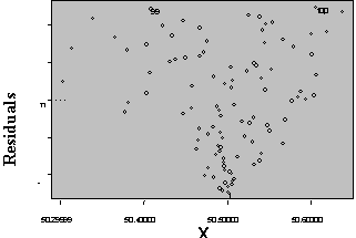
A frequent side benefit of improving non-linearity in the regression is that a parallel reduction in the error term results, improving MSE, and often improving the distribution of residuals.  Non-linearity is removed by performing transformations on the X’s.  The modeler must always be careful to consider the case when the distribution of residuals is not normal or heteroscedastic, in which case transformations on Y might be needed. In these cases Y should be transformed prior to transformations of the X’s. Common transformations for specific patterns in scatter plots are show in Figure 6.

Multi-collinearity

The presence of multi-collinearity or inter-correlation between independent variables introduces complications into the regression function. Independent variables are often highly correlated when observational data are collected. Problems in the regression arise when two highly correlated variables are included in a regression model together, or when a variable is correlated with an important variable omitted from the regression model.

 

 

 

 

When two variables are uncorrelated, they are said to be independent or orthogonal.  When two variables are orthogonal, and their correlation coefficient is zero, then their estimated coefficients will remain the same whether or not they are included in the model.  Typically variables are orthogonal only as a result of controlled experiments—in observational data independent variables are rarely orthogonal to one another.

Suppose a model was estimated with Y, X₁ and X₂, where the X’s are uncorrelated.  Suppose that the following regression functions were obtained:

1)   Y = 500 + (0.452) X1 + (72.6) X2

2)   Y = 75 + (0.452) X1

3)   Y = 700 + (72.6) X2

Thus, when variables are uncorrelated, their coefficients will be the same regardless of what other uncorrelated variables are included in the model.  This is a desirable result, since the analyst is confident that the coefficient associated with a particular variable is really a stable estimate of its effect on Y.

When variables are correlated, the results are not easily interpreted.  In fact, the following side effects to the regression occur:

1)       Multi-collinearity does not inhibit our ability to obtain a good fit to the data, nor does it prevent us from obtaining confidence intervals, etc.

2)       Multi-collinearity does, however, lead to large sampling variability of the individual regression coefficients, or inefficient estimates.   One can in fact end up with a significant F-ratio test, but insignificant t-tests for all individual variable coefficients

3)       Estimated regression coefficients cannot be directly interpreted when the variables are highly correlated, since it may be impossible to hold one constant while varying the correlated one.

4)       It is possible to get incorrect signs associated with coefficients when variables are highly correlated, especially when an independent variable is highly correlated with a variable omitted from the model.

5)       As the multi-collinearity increases, the ability to solve for the regression parameters becomes computationally difficult.

 

 

 

 

 

 

Fortunately, there are ways to diagnose multi-collinearity, and methods for remediation. The following are useful for diagnosing and remediating multi-collinearity.

1)       The simple correlation matrix provided as standard output in most regression packages is useful for identifying mutlicollinearity between independent variables. As a general rule of thumb, correlation higher than 0.7 or 0.8 should be checked. In addition, the variance inflation factor (VIF), provides an indication of how inflated the sampling variances of the parameters are due to multi-collinearity.

2)       The analyst can restrict the use of the regression function to cases where the co-linear independent variables follow the same co-linear structure as in the model. In other words, if the multi-collinearity exists in reality across time and space, then its effect on the regression might not create serious problems of representativeness of the real phenomenon.

3)       One or several correlated independent variables can be dropped from the model.  This creates two new problems, however.  First, it is difficult to obtain direct information about dropping the terms from the model.  The coefficients remaining in the model are affected by the correlated independent variables not included in the model.

4)       Apply Ridge Regression, which introduces a biasing constant into the standardized normal equations, resulting in a significant reduction in the inflated sampling variability due to multi-collinearity.  In this procedure, biased estimators of the beta’s are obtained, but the sampling variability is reduced, which might be preferred to an unbiased estimator (such as OLS) with large sampling variability.

Non-Constancy of Error Variance

Non-constancy of the error terms is a common occurrence in the practice of regression, and arises in many cases naturally. Recall that that VAR [Y_hat] = VAR [residuals] = s² for all predicted values of Y, and therefore for all X. Again, three plots to assess constancy of the error terms are employed.

1)       Residuals versus the independent variables,

2)       Residuals versus the fitted values, and

3)       Residuals squared versus fitted values (or independent variables).

Heteroscedastic (non-constant) errors occur fairly often with data and model development.  Consider, for example, if yearly vacation expenditures is the dependent variable.  One might expect much greater variability at higher household incomes than at the lower household incomes, since presumably higher income households have greater discretionary income in which to spend on vacation. Figure 6 shows how non-constant error can be detected through the use of various diagnostic plots.

Figure 6: Diagnostic Plots for Detecting Heteroscedastic Errors

 

       

             

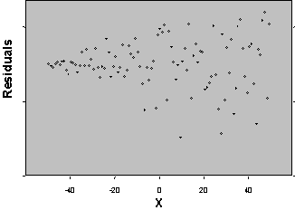
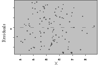
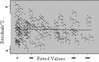
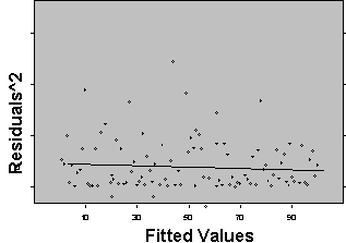
There are methods designed to minimize SSE for the linear regression based on a family of transformations on Y. The following represent transformations on Y that can be attempted to correct for heteroscedastic error terms. Figure 7 shows common transformations on Y and the pattern of residuals that accompany such needed transformations. For a comprehensive listing and detailed description of transformations and their effect on a regression relation, see Appendix B.

 

Figure 7: Transformations of Y for Correcting Error Heteroscedasticity

 

 

 

 

 

 

 

 

 

 

 

 

 

 

 

 

 

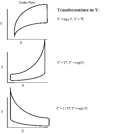
Independence of Errors

This is really appropriate for time-based observations, where the Yi’s were collected over evenly spaced time increments such as seconds, months, or years.  There can be many effects of time, including seasonal variation, time of day variation, learning processes, and adaptive processes, etc.  In essence, there should be little or no correlation between residuals over time in a regression model. In reality, however, time series observations often possess correlation over time, or serially correlated errors. A plot of residuals over time can reveal any problems with serial correlation.

There are methods developed to remediate serially correlated errors.  Time Series Analysis deals with the multitude of issues that arise with time series type data.

Presence of Outliers

Outliers are observations that exert extreme influence on the fit of the estimated regression function. Outliers are detected graphically through inspection of plots of standardized residuals (residual/ÖMSE) versus X or fitted Y.  Because of their great influence on the regression equation, outliers can create great difficulty with the regression function. There are several reasons for this.

1)       The outlying observations are outside the body or bulk of data, and therefore may represent anomalous data.

2)       If the regression function is heavily swayed by potentially anomalous data, the regression function may not do an adequate job representing the relationships embedded in the bulk of the data.

3)       Outliers may actually be the result of an error, such as mis-coding of data, poorly calibrated instrumentation, transcription error, etc., and thus should be corrected if possible.

4)       Outliers may represent a phenomenon that warrants further study, and therefore these observations need to be scrutinized more carefully.

Recall that in solving for the parameters of the regression, the sum of squared deviations is minimized.  When an outlier is present, therefore, it may unduly influence the fit of the regression function, leading to a significantly different fit had the outlier not been present. 

The analyst generally identifies ‘influential observations’ or outliers first, and then determines if they should be discarded, given a separate regression model, or left in the model as adequate representation of the phenomenon under study.  In general outliers should not be discarded unless one of the following conditions can be shown to have occurred:

1)       An error was made recording the data,

2)       A miscalculation was made in deriving the data,

3)       Measuring equipment was malfunctioning, or

4)       The outlying data points are unique in some identifiable way and deserve their own model.

If none of these reasons can be supported or justified with direct evidence, the general rule is to leave an outlier in the data set, assuming that it represents valuable information.

There are mathematical methods for identifying outliers, and quantifying their influence on the regression function.  The commonly used methods include DFFITS, DFBETAS, and COOK’s measures. A simple plot of the standardized residuals vs. X (see Figure 8), or residuals versus X or fitted Y can reveal the presence of outlying observations in a regression.

 

 

Figure 8: Plot of Standardized Residuals vs. X for detecting Outlying Observations

 

                                                                Non-Normality of Error Terms

 

 

 

 

 

 

 

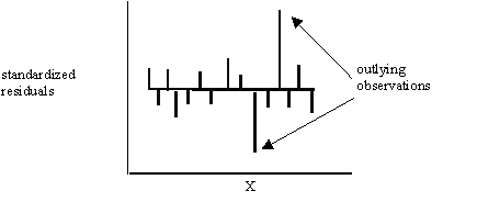
Moderate departures from error-term normality do not create serious problems for the regression.  However, serious departures from normality are of concern. The normality of error terms can be studied both graphically and quantitatively.

Several plots are useful for assessing the distribution of errors. They include box plots, histograms, and normal probability plots.  The Boxplot and histogram is shown in Figure 9.  In the box plot and histogram the analyst looks for symmetry about the mean, or 0, and look for the presence of outlying observations. The plots in the figure represent data that are normally distributed.

The normal probability plot shows how a normal population versus the observed data would plot on the graph. An ideal fit would be a diagonal line on the plot.  Large departures suggest non-normal errors, while small departures suggest normality. These plots are provided in most standard regression software packages.

There are formal methods for examining the normality of errors.  For example, one can compute the correlation coefficient between expected (under normality) and observed residuals.  For a given alpha level, the analyst can compute the correlation coefficient and test whether or not the residuals are likely to come from a normal distribution.

When the errors are not normally distributed, one cannot make inferences based on the regression function.  For example, confidence and prediction intervals cannot calculated with accuracy.  The options for correcting non-normality of the residuals are several. First, transformations of Y can be used to normalize the residuals. Second, the ‘correct’ distribution can be identified, such as Poisson, Gamma, or negative binomial, and generalized regression models can be used. Finally, in the case of an unidentifiable distribution of errors, Monte Carlo techniques can be employed to develop confidence and predictions intervals.

 

Figure 9: Box Plot and Histogram Depicting Normality of Regression Residuals

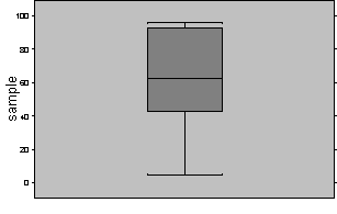
            Normality of Residuals                                                    Non-Normality of  Residuals

                                                                 

 

 

 

 

 

 

 

 

 

 

 

 

                                                     

 

 

 

 

 

 

 

 

 

 

 

 

 

 

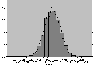
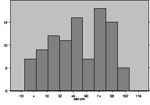
Omission of Important Independent Variables

There are times (although the researcher tries to avoid this in early stages of planning a research study) when critical variables were not used in the estimation of the model.  By plotting the residuals versus the excluded variable, whether it is a dummy variable or a continuous one, the analyst might observe a systematic trend in the residuals that might suggest that inclusion of that variable might improve the model.

As an example, consider the plot of residuals for an automobile emissions model versus the regression model fitted values, shown in Figure 10. Suppose that an omitted variable, number of engine cylinders=8, was suspected of being influential in the process of emission formation. When 8 cylinder engine vehicles only are plotted against the model residuals, as shown in the plot on the left, the residuals are generally positive for these vehicles, which demonstrates that observed emissions are always higher than predicted by the model for these vehicle types. Thus, the variable number of engine cylinders probably should have been included in the model as an indicator variable. Had the residuals been randomly distributed for vehicles with 8 cylinder engines, then there would not have been evidence to include it in the model. Of course, the inclusion of an additional variable would need to be scrutinized by all relevant model fit statistics, t-ratio, r-square, and F-test results.

 

Figure 10: Plot of Automobile Emissions Residuals vs. Regression Model Fitted Values

                               8 Cylinder Engines                                                                 All Vehicles

        

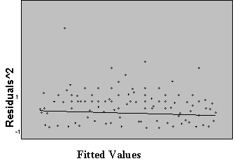
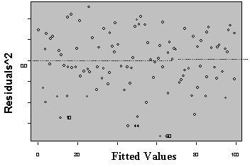
One or more of the X’s are influenced by the value of Y.

It is assumed that the model is structured such that Y is dependent upon values of the X’s. In other words, the direction of influence is assumed to flow from right to left in the equation—the right-hand-side variables influence Y. The X’s, on the other hand, should not be influenced or determined by Y. Right-hand-side variables that are determined ‘outside’ the model are called exogenous, and those that are determined by Y are called endogenous. Standard regression techniques assume that all right-hand-side variables are exogenous. Endogenous variables must be dealt with using somewhat advanced techniques such as instrumental variables or structural equation models. For further reference see Greene, 1997, or most textbooks on econometrics.

The independent variables (X’s) in the model are assumed to have been measured without error.

In the standard ordinary least squares regression model it is assumed that Y is measured with error, and this is partly what contributes to the difference between observed and predicted Y. The presumption, however, is that the X’s are measured precisely. That is measurement error in the X’s can largely be ignored because it is small. When measurement error in the X’s is large, one must consider alternative methods of model estimation. The most popular of measurement error models are structural equation models. Other software packages are available for handling measurement error problems.

Refine the Regression Model

After the modeler has iterated between different models, checking the requirements of the regression, making necessary transformations, then re-estimating models, she is now ready to make final refinements to the model. In this stage multi-collinearity problems and goodness of fit of the ‘best’ model specifications are assessed.

Recall that the analyst must consider the objectives of the research and resultant model, and the variables that have been considered in the model. The first model inspection should consist of checks on the variables in the models, including interaction effects, higher order interactions, and whether the model makes sense from theoretical grounds. Then, some statistical measures can be used to refine the models, and compare and contrast various “good” model formulations.           

Descriptive Measures of Association Between X and Y

Models are assessed and refined using measures of association between X and Y. The most common descriptive measures are R-Square, commonly called the coefficient of determination, and the coefficient of correlation, r.

The coefficient of determination is defined as:

where;

R² is the coefficient of determination,

SSTO is the total sum of squares,

SSR is the sum of squared regression,

SSE is the sum of squared errors,

and 0 £ r² £ 1.

The coefficient of determination R² can be thought of as the proportionate reduction of total variation associated with the use of the independent variables, or X’s. Commonly it is interpreted as the proportion of total variance explained by the X’s. When SSE = 0, R² = 1, and all of the variance is explained by the model. When SSR = 0, R² = 0, and there is no association between the model X’s and Y.

Because R² can only increase with additional variables in a model, an adjusted measure, denoted R²_adjused accounts for the degrees of freedom changes as a result of different numbers of model parameters, and allows for a reduction in R²_adjusted. The adjusted measure is superior for comparing models with different numbers of parameters.

It is common to place too much emphasis on the R² measure or to mis-interpret it. The measure is only relevant to compare against previous studies that have been conducted on the phenomenon under investigation. Thus, an R²_adjusted of 40% in one study may be considered “good” only if it represents an improvement over past studies and the improvement reflects a real contribution to an understanding of the underlying phenomenon. Thus, it is possible to obtain an improvement in the R²_adjusted value without gaining a greater understanding of the phenomenon being studied. It is only through the combination of a “good” R²_adjusted value and a material understanding/explanation of the phenomenon that refines an existing understanding of an underlying data generating process.

Finally, it should be noted that the R²_adjusted value is bound by 0 and 1 only when an intercept model is applied. When the intercept is forced through zero the R²_adjusted value can exceed the value 1 and is not as useful for comparisons across models.  

The coefficient of correlation r is the square root of R². It is more commonly used to express the linear association between two variables, and not multiple variables in the regression. The coefficient of correlation can be computed as follows: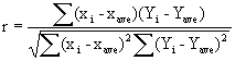

where the slope of the regression functions determines the sign.

Other measures are available for assessing and comparing model fits. These include comparisons of Mean Squared Error (MSE), Mallow’s CP, and other similar measures.

     

Validation of the Regression Model

Internal and external validation of the regression model are critical steps in the model building process. Validation is perhaps the most often overlooked aspect of model building. This is unfortunate, since validation is the most objective method to assess the credibility of a model. There are several important reasons to validate a model.

1)       The process of fitting a statistical model to data can result in anomalous fits to the data. In essence, apparent relationships reflected through significant variables are the result of over-fitting and not real relationships that generated the data. For further information see Myers, 1990, pp. 178-180. 

2)       It is important to ensure that the sampling frame chosen for the population of interest will yield a sample that accurately represents the population. The poll that forecast Dewey as the next president in 1948 was wrong because of a sampling frame error.

3)       The theoretical expectations of the model should agree with empirical results obtained from modeling the sample data.

4)       Some of the relationships captured in the sample data may not be valid over time or at other locations.

To conduct model validation an independent set of data is needed. There are numerous ways to generate data for model validation, three of which are described here.

1)       A holdout data set is retained from the original data. Thus, in planning the sample size for the study, the size of the sample should be increased by an additional 20%, for example. The data should be collected as usual. When it comes time for model building, a random sample of 20% can be removed from the model-building data set, and used for validation purposes. If data were collected over time or were collected in pairs, then data could be split over time or pairs could be split to determine if these factors would render model extrapolations invalid. If there are no perceivable differences between the holdout dataset and the estimation sample, then the validation merely can be used to determine if the model was over fit to the estimation data (i.e. spurious relationships were detected). If the holdout data represents a study replication, then the validation will also test the generalizability over time and space.

2)       A second alternative it so collect additional data after the initial data collection effort. However, this is impractical in some studies, as it usually more expensive to collect data after the initial data collection effort. There are times, however, when other efforts may collect similar data, and these should be viewed as opportunities for model validation.

3)       A third procedure for model validation involves computer programming via Monte Carlo methods. Essentially, the data are randomly assigned to 10 bins, resulting in 10% of the data assigned to each bin. Then the first 10% is removed from the data and used for validation on the model estimated using the remaining 90%. The 10% are then returned to the data and the 2^nd 10% are removed, and a new model estimated on the remaining 90%. This process is repeated 8 more times to complete the analysis. This process results in an efficient use of the data, because all the data are used to estimate models and all the data are used for validation. The results can be presented for each of the 10 model estimations and validations, and assessments can be made as to the validity of each of the drawn samples. Again, this technique is most useful for checking for model over-fitting of the model to data. Similar methods include the PRESS statistic and other re-sampling methods.

There are numerous measures of goodness-of-fit used to compare model predictions to actual data in the validation process. The sum of squared prediction errors, the mean squared prediction error, the mean absolute prediction error, and Thiel’s U-statistic, the Press Statistic, and Conceptual Predictive Criteria (C_p Statistic) are examples of methods that can be used to compare model predicted results to validation data.

Conduct statistical inference, document model, and implement

The modeler is now ready to conduct statistical inference, document the model, and implement. Statistical inference is the process by which inferences are made about the population, or process being modeled, based on the model estimated on the sample of data. Statistical inference is the cornerstone of statistical theory and allows the modeler to make statements about the population.

There are several estimated parameters that are used to make inferences about the population, the betas, which represent the mean change in Y given a unit change in the X, and Y_hat, which reflects the mean response given a combination of X values. Each of these is discussed here.

Inferences on b’s

Inferences surrounding the betas in a regression are useful in that information can be obtained as to the uncertainty in the effect of an individual X on Y. It can be shown that: 

           An unbiased estimator of the variance of b₁ is given by: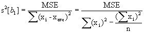 

The square root of s², s [b1] is the estimator of s[b1].

A useful distribution that arises in statistics is the students’ t distribution, which is the ratio of (X_ave - m) to Ö(S²/n).  It can be shown that s (b₁) is t distributed with n - p degrees of freedom, where n is the sample size and p is the number of estimated parameters.

A confidence interval for b₁ is given by: 

where;

t is percentile of the t distribution,

a is acceptable confidence error in decimal, i.e. .01, .05,.10 etc, and

n - p are the appropriate degrees of freedom.

The interpretation of a confidence interval is very explicit and should be treated with caution.   A 1- a confidence interval on b₁ indicates that the true value of b₁ will fall within the confidence limits given repeated samples taken on the same X levels a times out of 100.  Recall that b₁ is the mean change in the mean of the distribution in Y with a unit change in x.

 

One-sided versus two-sided hypothesis testing

The confidence interval given by b₁ +- t {1 - a / 2;  n - 2} s [b₁] is a two-sided confidence interval.  This means that the analyst is concerned with how probable events are on either side of the true parameter b₁.  Often, the engineer wants to ask the question “does some confidence interval of b₁ contain the value 0?”  The alternative hypotheses then are:

            H_0:  b₁ = 0, and H_a: b₁ ¹ 0.

 

If the confidence interval for a given confidence level 1 - a (i.e. 1 - .05 = .95) does not contain 0, then one can conclude that at that confidence level, a*100 times out of 100 when repeat samples are drawn at the same x levels the confidence interval will not contain 0.

The analyst could alternatively test whether b₁ is positive.  In this case the test hypotheses are:

            H_0: b₁ £ 0, and H_a: b₁ > 0.

 

In this case one side of the distribution is considered such that all the error is assigned to one side of the probability distribution.

 

Confidence Band around Regression Function

Often an analyst is concerned with quantifying the confidence in the mean response around the entire regression function. To accomplish this, a procedure that allows for multiple simultaneous tests on the fitted regression line is used. In other words, the confidence interval is appropriate for many research questions ‘asked’ about the regression function. One method is the Working-Hotelling approach, which for a 1 - a confidence band around the regression function has the following two boundary conditions at X_h: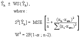                                                                                                                                                                                     

This simultaneous confidence band around the regression function is a wider confidence interval at X_h than that computed by a single confidence interval estimate at X_h.

 

Model Documentation

Once a model has been estimated and selected to be the best among competing models it needs to be thoroughly documented, so that others may learn from the modeler’s efforts. It is important to recognize that a model that performs below expectations is still a model worth reporting. This is because the accumulation of knowledge is based on objective reporting of findings—and only presenting success stories is not objective reporting. It is just as valuable to learn that certain variables don’t appear effectual on a certain response than vice versa.

When reporting the results of models, enough information should be provided so that another researcher could replicate your results. Not reporting things like sample sizes, manipulations to the data, estimated variance, etc., could render follow-on studies difficult.

Perhaps the most important aspect of model documentation is the theory behind the model. That is, all the variables in the model should be accompanied by a material explanation for being there. Why are the X’s important in their influence on Y? What is the mechanism by which X influences Y? Would one suspect an underlying causal relation, or is the relationship merely associative? These are the types of questions that should be answered in the documentation accompanying a modeling effort. In addition, the model equations, the t-statistics, R-square, MSE, and F-ratio tests results should be reported. Thorough model documentation will allow for future enhancements to an existing model.

Model Implementation

Model implementation, of course, should have been considered early on in the planning stages of any research investigation. There are a number of considerations to take into account during implementation stages:

1)       Are the variables needed to run the model easily accessible?

2)       Is the model going to be used within the domain with which it was intended?

3)       Has the model been validated?

4)       Will the passage of time render model predictions invalid?

5)       Will transferring the model to another geographical location jeopardize model accuracy?

These questions and other carefully targeted questions about the particular phenomenon under study will aid in an efficient and scientifically sound implementation plan.

How is a regression equation interpreted?

A regression equation represents the linear additive association between a dependent variable Y and one or more independent variables (X’s). The regression parameters, or partial slope coefficients, represent the change in Y given a unit change in X, all else held constant. If the regression was estimated using experimental data, then the regression parameters represent the change in Y caused by a unit change in a particular X. If the regression was estimated using quasi-experimental or observational data, then the regression parameters represent the change in Y associated with a unit change in a particular X.

The regression equation is meant to model as accurately as possible the relationships in the true population, in as simple an equation as is possible. The regression model is known not to capture all the structure in the real data, and is known to be wrong to some degree. The model represents a convenient way to explain relationships or predict future events given known inputs, or value of the independent variables (X’s).

How do continuous and indicator variables differ?

Continuous variables are usually interval or ratio scale variables, whereas indicator variables are usually nominal or ordinal scale variables. Indicator variables can be entered in the regression to adjust the y-intercept term, or be interacted with a continuous variable and affect the slope coefficient of the interacted variable. Indicator variables are somewhat analogous to testing the difference in means between two groups as in ANOVA. Indicator variables in the regression can only take on one of two values— 0 or 1. 

How are partial slope coefficients interpreted?

The beta’s in a regression function are called the regression coefficients, or partial slope coefficients in multiple independent variable regression. 

The meaning of the parameter b₀, indicates the mean of the probability distribution at x = 0, if a distribution exists at x = 0.  When x = 0 does not exist, b0 does not have any particular interpretation or meaning.

The coefficient with the variable, b₁, indicates the change in the mean of the probability distribution of Y per unit increase in X, considering their difference in units. If the independent and dependent variables are standardized, then the partial slope coefficients are in the same standardized units.  If the regression coefficients in the model were estimated on the X’s in their original units then the magnitude of coefficients across X’s cannot easily be compared; however they are meaningful in that the analyst can assess unit changes of individual variables in their original ‘intuitive’ units. Standardized regression coefficients, calculated on standardized variables, offer an advantage over non-standardized variables in that the magnitude of effects can be compared on standardized units. For further discussions consult Neter et al. (1990, 1996) and Myers (1990).

What are interactions?

Interactions are often important effects that need to be considered in the regression. In the standard regression model without interaction terms the effect of X₁ on Y depends only on the level of X₁, and is equal to bX₁.  Suppose, however, that the effect of X₁ on Y depended not only on the level of X₁, but also on the level of X₂. This multiplicative effect is called an interaction between X₁and X₂.      

An interaction between two variables is called a second-order interaction, between three variables is called a third-order interaction, etc. A variable in a model non-interacted with other variables is called a main effect. In general main-effects are more important with respect to ‘explaining variability’ than interactions, and the higher the order of interaction the less influential the effect is on Y. Interactions, however, may reflect important aspects of underlying data generating processes, and therefore may be kept in the model on these grounds alone, and not on the basis of their contribution to the R² value.

What are standardized regression coefficients?

Standardized regression coefficients are obtained by performing regression on standardized variables. Standardized variables result from transforming an original X by subtracting the mean of X and dividing by the standard error of X, such that X_s=(X-X_ave)/s_X. When standardized variables are used in a regression their partial regression coefficients can be compared across the independent variables.

How is the F-test interpreted?

The F-test is a general test that can be used in a myriad of ways to test regression models. In essence, the F-test compares the results of two models to one another to see if the more complex (full) model is convincingly better than a simpler (reduced) model. The standard F-test provided in many statistical program output compares the explanatory power of the full model to the reduced model with only the y-intercept term in it, which is equivalent to the sample mean. Thus, it compares a model with one or more partial slope coefficients to the sample mean model, to see if it provides a convincingly better fit to the data.

How are t-statistics interpreted?

A t-statistic is similar to an F-test, except the test is for a single variable in the model. The standard t-test provided by most standard statistical software packages is used to determine the probability that an individual variable’s parameter is equal to zero. In actuality the test is conditional on the variable’s parameter equaling zero, and provides the probability of the data having arisen under this constraint.

How are r and R² interpreted?

The correlation coefficient (r) and coefficient of determination (R²) are two measures of model goodness of fit. These two measures are related in that (r)² = R². The R-squared value is the variance explained by the model divided by the total variance, both explained and unexplained. High R-squared values indicate that a model explains a large portion of the data variability, while a low R-squared value indicates the opposite. R-square values cannot be compared across models with different numbers of variables. An adjustment to R-square is needed to make fair under these circumstances. R-squared values shouldn’t be compared across different phenomenon, either. For some phenomenon an R-squared value of 0.35 represents a very good model, whereas for some others an R-squared value of 0.85 represents a poor fitting model.

R-square values are commonly abused measures of model fit, as they often become the only method for variable selection. This practice is ill advised. Variables should be selected based on their theoretical and practical appeal and appropriateness, not merely because they contribute to a higher R-squared value. The practice of data mining in modeling to improve R-square is not grounded in science, and should be avoided to the extent possible.

How are confidence intervals interpreted?

A confidence interval is interpreted as follows: If samples were repeatedly drawn at the same X-levels as were drawn in the original sample, then alpha (a) times out of 100 the mean of the sample Y’s will fall within the (1-a)% confidence interval. In simpler but less technically correct terms, the analyst is (1-a)% confident that the mean of a new sample falls in the confidence interval.

How are prediction intervals interpreted?

A prediction interval is interpreted as follows: If samples were repeatedly drawn at the same X-levels as were drawn in the original sample, then alpha (a) times out of 100 an individual observation of Y will fall within the (1-a)% prediction interval. In simpler but less technically correct terms, the analyst is (1-a)% confident that an individual observation would falls within the prediction interval.

How are degrees of freedom interpreted?

Degrees of freedom are associated with sample size. Every time a statistical parameter is estimated on a sample of data the ability to compute additional parameters decreases. Degrees of freedom are the number of independent data points used to estimate a particular parameter.

 

Should interaction terms be included in the model?

Interaction terms represent potentially real relationships embedded in data. Most often they arise in quasi-experimental and observational data. An interaction that is important should be included in the model, despite the fact that it might not contribute much to R-square. In general, third and higher order interactions (that are real in the population) can be ignored without much detriment to the model.

How many variables should be included in the model?

The objective of most modeling efforts is to economize the model. In other words, the analyst generally wishes to explain as much of the data complexity with as few variables as practicable. Generally seven variables plus or minus two variables covers most models, although smaller and larger models can be found. It is generally better to favor a simpler model to a more complex one, simply because interpretation and implementation are simplified also. On the other hand, if the phenomenon is sufficiently complex, then making too simple a model may sacrifice too much explanatory or predictive power.

What methods can be used to linearize the regression relation?

Transformations of the X’s are used to linearize the relation between Y and X’s.  Common transforms include the log base ten and natural logs, inverse logs, powers, roots, and reciprocal functions. The nature of the non-linearity can often be inspected to determine which transform will be most useful.

What methods are available for fixing heteroscedastic errors?

Heteroscedasticity, a fancy term for non-constant variance, is a violation of the OLS regression and needs to be fixed, or other methods need to be employed. The standard procedure is to transform Y using log base ten and natural logs, inverse logs, powers, roots, and reciprocal functions. Pre-caution should be taken, however, because transforming the response variable often makes the response counter-intuitive, or difficult to interpret. The solution is of course to transform back to the original response after the regression is estimated. Another precaution is that transforming Y often makes the relation with X’s non-linear, so parallel transforms for the X’s are also needed. The modeler should always keep in mind that transformations on Y are for purposes of meeting the modeling theory, and the natural units of the response are often the most interpretable and intuitive.

What methods are used for fixing serially correlated errors?

Serially correlated errors occur with time-series data. That is, the researcher might have data that were collected over time, such as strain gauge tests on a bridge at one-year intervals. If there is dependence of Y across time, then the errors will be serially correlated. Time series analysis, which is a natural extension of regression, is the method for fixing serially correlated errors.

What methods are used for fixing correlated errors?

Correlated errors arise when one or more X’s in a model is directly related to another X (or X’s) in the model, or Y. Suppose X₁ is largely determined by X₂, and both these variables are in a model to predict or explain Y. Since X₁ is simply the sum of X₂ times a constant plus an error term, then the error component of the model is correlated across observations, which is a violation of one of the assumptions. The solutions for this problem involves first detection of the problem, and second identifying a remedial measure. Detection of the problem is best done through intimate knowledge of the data and how they arose. It should be clear that none of the X’s is largely determined by the other X’s. Associations between variables are not a problem (it can cause multi-collinearity, which is a different problem), however direct causality between them is. The solution is to go to simultaneous equations models, such as two-stage and three-stage least squares procedures.

What can be done to deal with multi-collinearity?

Multi-collinearity is when two variables co-vary, and is common in non-experimental data. It is not a violation of the regression model explicitly, however it causes problems in the mathematics of solving for the regression parameters. In essence, highly collinear variables (e.g. a correlation coefficient of 0.7 or higher) cause regression parameters to be inefficient (high standard errors), and can cause the signs of the regression coefficients to be counter-intuitive.

There are several remedies to the multi-collinearity problem. First, the variables can be left in the model and assumed to reflect the natural state of those variables in reality, and so accepting of the ever-present collinearity. A second option is to remove the less important of the two collinear variables and keep only one in the model. This is usually the preferred option. The third option is to employ a structural equation modeling approach instead of regression. Structural equations models explicitly use covariance among variables in the model building process. Finally, Ridge Regression may be applied.

What is endogeneity and how can it be fixed?

Endogeneity is fancy term for having an independent variable that is directly influenced by the dependent variable Y. It is presumed a priori that all independent variables are exogenous—that they are determined by influences outside of the modeling system. When a particular X is endogenous, the model errors are correlated with the variable (see correlated errors FAQ), and problems in the regression occur, such as biased estimates, etc. Some remedies include the use of instrumental variables approaches, proxy variables, and structural equations models.

 

 

Time Series Analysis is used to develop forecast models for time-indexed data.  The theory and application of time series analysis come primarily from the field of econometrics.  Economists established econometrics in the early 1930s when “an unprecedented accumulation of statistical information” was creating “a need to establish a body of principles that could organize what would otherwise become a bewildering mass of data.” (Greene, 1997).  Transportation engineers and planners face the same challenge today.  Time Series Analysis provides a powerful set of tools to leverage transportation system data for improved system planning, management and control.  Two types of univariate time series models are presented in this section: exponential smoothing models and autoregressive integrated moving average (ARIMA) models.

6)       The random component of the data series is uncorrelated with zero mean and constant variance.  The term for such a series is white noise.  The instances of white noise disturbance in the data series are called innovations.

7)       Either the raw time series data or some transformation of the raw data must satisfy the following three conditions –

·         the unconditional expected value of the observations in the series is constant with respect to time

·         the variance of the observations is constant with respect to time

·         the covariance between any two observations in the series depends solely on the time lag between the observations (i.e., not on the time of occurrence of either observation)

This requirement is referred to as weak stationarity.

Time indexed data series with observations taken at discrete intervals .

Sample of n observations on , i.e. .

 

Sample estimate of the variance of .

A parameterized model for  in terms of previous observations and/or innovations.

 

 

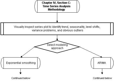
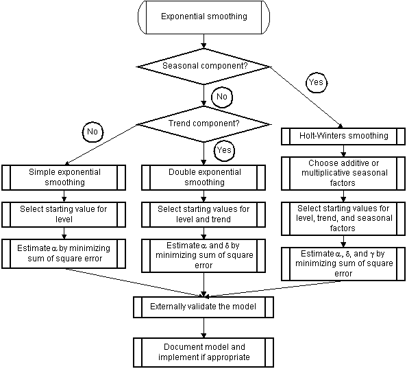
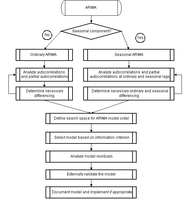
Planning Forecasts

Nihan, N.L. and K.O. Holmesland (1980). Use of the Box and Jenkins Time Series Technique in Traffic Forecasting. Transportation, vol. 9, pp. 125-143.

Operational Forecasts

Ahmed, M.S. and A.R. Cook (1979). Analysis of Freeway Traffic Time-Series Data by Using Box-Jenkins Techniques. Transportation Research Record #722 pp. 1-9. National Academy of Sciences.

Ross, P. (1982). Exponential Filtering in Traffic Data. Transportation Research Record #869 pp. 43-49. National Academy of Sciences.

Williams, B.M., P.K. Durvasula and D.E. Brown (1998). Urban Freeway Traffic Flow Prediction: Application of Seasonal ARIMA and Exponential Smoothing Models. Transportation Research Record #1644 pp. 132-141. National Academy of Sciences.

 

How is a time series model equation interpreted?

How is the variance estimate interpreted?

How are prediction intervals interpreted?

How are information criteria interpreted?

Are there ARIMA equivalents to exponential smoothing models?

What methods can be used to detect and model outliers?

What if the errors are not white noise?

Box, G.E.P. and D. Cox. (1964). “An Analysis of Transformations.” Journal of the
Royal Statistical Society, Series B, 389-398.

 

Box, G.E.P. and G.M. Jenkins. (1976). Time Series Analysis: Forecasting and Control, Revised Edition, Holden-Day, San Francisco.

 

Brockwell, P.J. and R.A. Davis. (1996). Introduction to Time Series and Forecasting, Springer-Verlag New York, Inc., New York.

 

Chang, I., G.C. Tiao, and Chung Chen. (1988). “Estimation of Time Series Parameters in the Presence of Outliers.” Technometrics, 30, 193-204.

Chatfield, C. and M. Yar. (1988). “Holt-Winters Forecasting: Some Practical Issues.” The Statistician, 37, 129-140.

Chen, Chung, and L. Liu. (1993a). “Forecasting Time Series with Outliers.” Journal of Forecasting, 12, 13-35.

Chen, Chung, and L. Liu. (1993b). “Joint Estimation of Model Parameters and Outlier Effects in Time Series.” Journal of the American Statistical Association, 88, 284-297.

Ljung, G.M. and G.E.P. Box. (1978). “On a Measure of Lack of Fit in Time Series Models.“ Biometrika, 65, 297-303.

Yar, M. and C. Chatfield (1990). “Prediction Intervals for the Holt-Winters Forecasting Procedure.” International Journal of Forecasting, 6, 127-137.

Visually Inspect Series Plot to Identify Trend, Seasonality, Level Shifts, Variance Problems, and Obvious Outliers

A thorough visual inspection of the data is essential.  The analyst will be specifically looking for evidence of trends, seasonal patterns, abrupt level shifts, variance changes, and gross outliers.  For example, Figure 11 illustrates the clear and expected weekly pattern in two weeks of freeway flow rate data (the plot is fourteen consecutive days of 15-minute hourly flow rates beginning with Sunday).  Unexpected or counterintuitive features should also be noted.

 

Figure 11: Two Week Traffic Flow Rate Plot Showing Recurrent Weekly Pattern

 

Figure 12 presents a classic data set from time series literature (Box and Jenkins, 1976).  The data are monthly international airline passenger totals from January 1949 to December 1960.  Inspection of the upper plot reveals a trend, a yearly pattern, and an increasing variance.  In the lower plot, a natural log transform has been used to address the increasing variance.

Figure 12: Monthly Airline Passenger Data

The general approach to dealing with non-constancy in variance is to apply what is referred to as a Box-Cox transformation on the input data (Box and Cox, 1964).  If we let  be the transformed series and  be the input series, the transformation is defined as:

Although l can be treated as real number parameter and estimated based on the sample data, in practice time series transformations are usually made by taking the natural logarithm () or taking the square root ().  The transformation is valid for all values of l only if  is strictly positive.  For example, the two common transformations just mentioned will not work on negative values.  Therefore, a preliminary transformation is required to use a Box-Cox transformation with a series that includes negative valued observations.  Most of the available software packages provide easy implementation of Box-Cox transformations, including automatic conversion of the forecasts back to original units.

 

Level shifts may indicate an abrupt change in the underlying process or processes generating the data.  For example, the return of students to a small college town would result in a marked increase in traffic flows in the area.  Two basic options are available when faced with level shifts in a continuous sample of time series data.  Either the level shifts can be modeled in the context of the overall sample, or the sample can be split into smaller samples at the shift points.

Outliers in time series data can result from either truly aberrant observations or from gross errors in the system that detects and records the data.  For example, a freeway accident that caused complete closure of all travel lanes would create outlying observations at downstream detection stations.  On the other hand, faulty detection equipment could also yield outlying data points.  Figure 13 shows one week of freeway traffic flow rates where the data collection system was “stuck” on 540 vehicles per hour for eleven hours.

Figure 13: Traffic Flow Rate Plot Showing Data Recording Outliers

The steps for dealing with outliers, trends and seasonal patterns depend on whether the time series analysis is based on exponential smoothing or ARIMA.  Missing values may also be present in the time series samples.  The method for handling missing values also depends on the model choice.  Modeling approach selection is the next step.

Select Modeling Approach

The time series model choice often depends more on the intended use of the forecasts than it does on particulars of the data series.  Therefore, this decision is likely to have already been made.  Nevertheless, if the information gathered during the visual inspection has relevance to the issue, this point in the process is a good time to revisit and reaffirm or change the selection.

Exponential smoothing was developed in the 1950s as an ad hoc forecasting approach.  However, a theoretical justification as well as a relationship to ARIMA was discovered after the fact.  Exponential smoothing is popular for many reasons.  It is easy to understand and intuitively pleasing.  Exponential smoothing methods have few parameters by definition and therefore avoid the pitfall of overfitting to the sample data with excessively complex models.  Exponential smoothing has proven to provide very good forecasts for a wide variety of univariate forecasting applications.

On the down side, exponential smoothing assumes a model form a priori.  Although the forecasts are likely to be reasonably good, a fitted exponential smoothing model will fully exploit the temporal correlation structure of the data only if the chosen exponential smoothing model form closely approximates the “true” underlying model form.

ARIMA on the other hand is a very general modeling framework.  The flexibility of ARIMA enables more accurate modeling but also opens up the potential for overfitting.  However, the use of model selection metrics known as information criteria help reduce the risk of overfitting and can even result in models that are simpler than exponential smoothing.  ARIMA in most cases will provide a more accurate model and in turn provide a better estimate of the series variance and better forecasts.

On the down side, ARIMA models require more expertise to develop.  Therefore from a field application standpoint, the marginal improvement in accuracy of ARIMA over exponential smoothing may not justify the added effort in some situations.

From a scientific research perspective, ARIMA clearly gets the nod.  Of the four principal types of exponential smoothing – simple, double, additive Holt-Winters, and multiplicative Holt-Winters – only multiplicative Holt-Winters does not have an equivalent ARIMA model representation.  Therefore, there is nothing to be lost from selecting ARIMA.  On the contrary, ARIMA provides a rigorous statistical framework in which to better understand the time-correlated nature of the data.

All this having been said, an analyst may choose to delay this decision altogether and develop a “best” exponential smoothing model and a “best” ARIMA model.  Given the ease of use of the available time series analysis software, the marginal effort to do both versus choosing one should be minimal.

Exponential Smoothing

The type of exponential smoothing used depends on whether or not the series in question has a characteristic seasonal pattern and /or trend.  If a seasonal pattern exists then one of the Holt-Winters methods must be used.  If a trend is present but a seasonal pattern is not, then double exponential smoothing is appropriate.  Simple exponential smoothing is for series with no trend or seasonal pattern.

Exponential Smoothing: Seasonal Component?

Seasonality in time series is usually known with a high degree of certainty before hand.  The traffic flow rate and airline passenger data in Figure 11 and Figure 12 above are examples.  In these types of series we expect our visual inspection of the data to confirm our hypothesis.  The visual inspection of seasonal data plots also give information on the stability of the recurrent pattern.  Holt-Winters exponential smoothing is indicated when a seasonal pattern is confirmed.

Exponential Smoothing: Trend Component?

As with seasonality, the presence of trend in a time series should be expected.  The obvious trend in the airline passenger data in Figure 12 mirrors the significant growth of schedule air travel during the 1950s.  Double exponential smoothing is indicated when there is trend but no seasonal pattern.

Exponential Smoothing: Simple Exponential Smoothing

Simple exponential smoothing is a single parameter forecast model appropriate for level, non-seasonal time series.  The recursive one-step forecast equation is given by:

where  is the level smoothing parameter and

 is the forecast of  from .

The recursions are equivalent to the following series:

The series representation shows that the forecast given by the recursive equation is equivalent to an exponentially weighted moving average of all current and past observations (hence the name “exponential smoothing”).  The rate of decay of the exponential weighting is governed by .

Future forecasts “flat line” in simple exponential smoothing for large t.   In other words, the forecast for time  is an estimate for the forecast for all times , where .

Reference was made above to an “after the fact” theoretical justification for exponential smoothing.  Specifically, it was proven that exponential smoothing is the limiting result as  of the exponentially weighted least squares solution for a constant level stochastic series.

Exponential Smoothing: Select Starting Value for Level

Since the recursive smoothing (forecast) equation requires both an estimate and an actual value, a decision must be made on how to “start” the recursions.  There are two basic choices.  If we give the first observation in the sample a time interval index of 1, i.e., , then we can either

·         let  be the forecast for the second interval  and begin the recursive forecasts at the third time interval

or

·         estimate the level at the time interval , take this estimate as , and use the recursive equation to calculate .

If the second option is used, the initial level can be calculated by averaging all the sample observations, averaging the first few observations, or fitting a line through the sample and using the value on the line at time .  The more consistent the level is across the sample, the less difference there will be among these three choices.  However, since there may be a general drift in the sample or in the first few observations, the latter two methods for estimating the initial level are more robust.  Most of available software packages allow analysts to either accept a default initial level calculation or input a user provided initial level estimate.  If the software default estimate is accepted, the analyst should be aware of how the initial level was calculated and be confident that the default estimate is appropriate.

A more precise way to estimate the initial level would be to reverse the sample, i.e.  becomes , use one of the methods above to begin the recursive forecasts on the reversed series, and take the estimate for  from the reversed series as  to begin the forecasts for the original series.  For simple exponential smoothing, this level of effort is rarely necessary.

Exponential Smoothing: Estimate  by Minimizing Sum of Square Error

The smoothing parameter is estimated by minimizing the sum of square error for the recursive forecasts.  If an Excel spreadsheet is used to generate the forecasts, the “Solver” tool can be used to do the estimation.   Another software option is the exponential smoothing routine in the statistical software package SPSS.  In SPSS, the user defines a range an increment for the smoothing parameter.  SPSS then calculates the sum of square error for each value of  in the range and reports back the ten values of  with the lowest sum of square error.

Handling of outliers and missing values can vary depending on the software used.  For example, if Excel is used, outliers and missing values can be replaced with the recursive estimates.  On the other hand, the exponential smoothing routines in SPSS were not designed to allow for missing values.  Therefore, SPSS requires the analyst to compute replacements for outliers and missing values prior to estimating the smoothing parameter.

When estimating replacement values for outliers and missing values, the goal is to derive reasonable values that do not bias the smoothing parameter estimates.  If the relative number of outliers and missing values is not high (say less than 10%, although this should not be considered a general rule of thumb), then the risk of model bias should be low.  In this case, simple techniques to calculate replacement values can be used, such as interpolating between reasonable observed values.  However, if the analyst is concerned with model bias, a more rigorous treatment of outliers should be considered.  Discussion of the available techniques would not be appropriate here.  However, references are provided in the response to the question – How extensive should the outlier analysis be? – in the trouble shooting section below.

Exponential smoothing: Double exponential smoothing

If a trend exists in a modeled time series that has no recurrent seasonal pattern, then double exponential smoothing is appropriate.  Double exponential smoothing is a two parameter model that includes a trend smoothing parameter, , in addition to the level smoothing parameter, .  Forecasts are calculated by the following set of recursive equations:

where  is the level smoothing parameter,

 is the trend smoothing parameter,

 is the forecast of  at time ,

 is the smoothed series level at time , and

 is the smoothed series trend at time .

As each successive observation is fed into the equations, the smoothed level is updated first, then this updated level is used to update the smoothed trend, and finally the updated level and trend are added to calculate the forecast for the next time interval.  The concept is exactly the same as in simple exponential smoothing except that now an interval-to-interval trend is being smoothed along with the level.

Exponential smoothing: Select starting values for level and trend

In double exponential smoothing, initial values must be estimated for level and trend.  Available options are similar to those for estimating initial level for simple exponential smoothing.

If we give the first observation in the sample a time interval index of 1, i.e., , then we can either

·         let , , and

or

·         estimate the level and trend at the time interval and add these together to calculate .

The level and trend at time  can be estimated by fitting a line through the entire sample or through some initial subset of the sample.  The initial level is the value on the line at time  and the initial trend is the slope of the line.  If the trend is not entirely consistent across the sample, using a subset of the first several observations may be more appropriate.

Exponential Smoothing: Estimate a and d by Minimizing Sum of Square Error

See the discussion of smoothing parameter estimation under simple exponential smoothing above.  The points highlighted for simple exponential smoothing apply for double exponential smoothing as well.  The only difference is that there are now two parameters to estimate.

Exponential Smoothing: Holt-Winters Smoothing

If the series of interest has a recurrent seasonal pattern then Holt-Winters smoothing should be used.  The full, three-parameter form of the additive Holt-Winters model is:

where  is the level smoothing parameter,

 is the trend smoothing parameter,

 is the seasonal factor smoothing parameter,

 is the forecast of  at time ,

 is the smoothed series level at time ,

 is the smoothed series trend at time , and

 is the smoothed additive seasonal factor at time .

The full, three-parameter form of the multiplicative Holt-Winters model is:

where  is the level smoothing parameter,

 is the trend smoothing parameter,

 is the seasonal factor smoothing parameter,

 is the forecast of  at time ,

 is the smoothed series level at time ,

 is the smoothed series trend at time , and

 is the smoothed multiplicative seasonal factor at time .

In both model forms, the parameter d in the seasonal factor subscript represents the length of the recurrent seasonal pattern in terms of number of time intervals.  For example, a series of monthly average daily traffic volumes would have a seasonal pattern that is 12 intervals long.  As the model is applied, there will be current values for the seasonal factor for each period within the seasonal pattern.  In other words, the monthly average daily traffic volume example would carry forward 12 seasonal factors, one for each month of the year.

The level and trend are updated at each time interval and used to generate the forecast for the next interval.  However, only the corresponding time period’s seasonal factor is updated at each time interval, and this updated seasonal factor will not be used for forecasting until the corresponding time period comes up again.  Going back to the monthly average daily traffic volume example, say we have just observed a new January monthly average.  This value will be used to update the level and trend for forecasting the February monthly average.  However, the seasonal factor used for the February forecast will be the one we updated last February, and the newly updated January seasonal factor will not be used until we are ready to forecast next January’s monthly average.

Exponential Smoothing: Choose Additive or Multiplicative Seasonal Factors

In the Holt-Winters framework, seasonal variation can be modeled either with additive or multiplicative seasonal factors.  In theory, the additive model carries the assumption that the seasonal effect is constant for each period in the seasonal pattern.  The multiplicative model, on the other hand, assumes that the seasonal effect at each period in the seasonal pattern is proportional to the local deseasonalized level.  After reflecting on these assumptions, it may be possible to make a defensible case for one model versus the other based on a priori knowledge about the process in question.

If the case is not strong for one method over the other, it might be prudent to develop both an additive and a multiplicative model and compare their performance.  If neither method emerges as a clear choice from a model accuracy perspective, the decision might hinge on practical considerations.  For example, for a strictly positive process whose values closely approach zero a particular points in the seasonal cycle, an additive model could result in negative forecasts.

Practical issues relating to Holt-Winters forecasting are not well covered in the available time series texts.  A paper in The Statistician titled “Holt-Winters Forecasting: Some Practical Issues” is a helpful reference (Chatfield and Yar, 1988).

Exponential Smoothing: Select Starting Values for Level, Trend and Seasonal Factors

Starting value selection is more critical for Holt-Winters forecasting than with simple and double exponential smoothing.  Since the seasonal factors are only updated once each cycle, they have less opportunity to adjust.  Therefore, poor initial choices for seasonal factors could have a significant effect on the seasonal smoothing parameter estimate.

Chatfield and Yar, 1988 group the options for starting value calculation into two classes global values and initial values.  Global values are based on all the data in the sample, and initial values are based on some subset at the beginning of series.  Chatfield and Yar recommend initial values.  Use of global values can result in underestimation of the smoothing parameters, especially the seasonal factor parameter.  Chatfield and Yar further recommend that either the initial values be based on backcasting or on the first two or three seasonal cycles.  Backcasting refers to reversing the data, using a simple method to calculate the initial values for the reversed series, and then using the forecast values at the end of the reversed series for the initial values for the original series.

The following example illustrates an initial value calculation based on the first three years of the airline passenger data given in Figure 12.  Since the seasonal effect appears to increase with level, multiplicative seasonal factors are appropriate.  In Figure 14 below, a fitted straight line is shown through the first three years of data.  The intercept of this line is 114 passengers.  This value can be used for the initial level.  The slope of the line is 1.7 passengers.  This can be used for the initial trend.

Table 11 presents the calculation of the initial seasonal factors.  The average of the first three years data is 145.5.  A ratio of observed passenger total to this average is computed for each of the first three years observations.  Finally, the three instances of each month are averaged.  It so happens that the calculated initial seasonal factors average to exactly 1.0.  When multiplicative seasonal factors do not average to 1.0 as first calculated, they should all be divided by the average.

Additive seasonal factors can be calculated in a similar fashion using the difference between observed and average values instead of the ratio.  Additive seasonal factors should sum to zero.  This is achieved by subtracting an equal allocation of the sum from each of the seasonal factors.

Figure 14: First Three Years of Airline Passenger Data

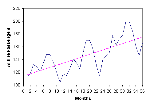
Table 2: First Three Years of Airline Passenger Data

 

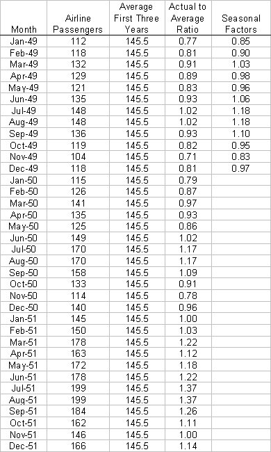
Exponential Smoothing: Estimate a, d and g by Minimizing Sum of Square Error

See the discussion of smoothing parameter estimation under simple exponential smoothing above.  The points highlighted for simple exponential smoothing apply for Holt-Winters smoothing as well.  The only difference is that there are now three parameters to estimate.

Exponential Smoothing: Externally Validate the Model

The fitted model should now be applied to a sample of data from the modeled series that were not used to estimate the parameters.  This is usually done by holding out a portion of the available data or by using a second sample separated in time from the one used to develop the model.  Goodness of fit measures can be compared to the results achieved on the model development data.  Although one would expect the fit to be better to the development data, the performance should not be markedly worse for the model evaluation data.

An often-overlooked step in model validation is to compare forecasts from the fitted model to naïve or heuristic forecasts.  For simple exponential smoothing, a reasonable naïve forecast to compare to would be .  For double exponential smoothing, one might compare the fitted model forecasts to .  Similar non-fitted heuristic forecasts can be developed for seasonal series as well.  If the fitted model cannot consistently outperform heuristic forecasts on the model evaluation data, then its usefulness is questionable.  Paired samples statistical tests such as the Wilcoxon Signed-Rank test can be used to assess the statistical significance of differences in performance based on absolute deviation or absolute percentage error.

Exponential Smoothing: Document the Model

The validated model should be thoroughly documented.  All assumptions should be clearly spelled out along with the rationale for any modeling decisions along the way.  Specific items to be documented include:

·         how outliers were handled

·         how initial values were selected

·         how the model parameters were estimated

·         the methodology and results of model validation

Exponential Smoothing: Implement the Model

Implementation of exponential smoothing models is very straightforward.  After initial values are calculated, the fitted recursive equations can be used to calculate on-line forecasts for the modeled data stream.

ARIMA

Autoregressive integrated moving average (ARIMA) models provide a general framework for modeling time correlated discrete time stochastic processes.  The autoregressive part of the term refers to a time series that can be represented in terms of past observations.  Autoregressive means “self-regressive” because the time series is in essence regressed on itself.  For example, a first-order autoregressive process would be represented as:

                                                where  is the autoregressive constant,

                                                 is the first order autoregressive parameter, and

                                                is the white noise innovation series.

The order of the process refers to how many steps back the model reaches.  A p-th order autoregressive process is referred to in shorthand as an AR (p) process.

Moving average refers to models that are expressed in terms past innovations instead of past values. For example, a first-order moving average process would be represented as:

                                                where  is the series mean,

                                                 is the first order moving average parameter, and

                                                is the white noise innovation series.

At first glance, the intuition behind moving average processes is not readily apparent.  However, the first order moving average process above can be rewritten as the following infinite series:

So the moving average process is an exponentially decaying function of the past series values.  A p-th order moving average process is referred to in shorthand as an MA (q) process.

Two useful time series conventions need to be presented before going forward with this brief introduction to ARIMA.  The first convention is the backshift notation.  The second convention is differencing notation.

The backshift operator is defined by the expression:

.

For example, .

Differencing creates a transformed series that consists of the differences between lagged raw series values.  The single lag difference operator is often denoted by the symbol .  Using this symbol, the first and second differences for the time series  can be defined as:

 .

Differencing with the single lag operator  is sometimes called ordinary differencing.  Differencing can also be applied at a seasonal lag.  For a series with a seasonal cycle of 12 intervals, the first seasonal difference would be defined as .

Using the backshift operator, the first difference can be written as , the second difference as , and so on.

The “I” in ARIMA refers to differencing necessary to achieve stationarity.  We can now introduce the general ARIMA model.

ARIMA Process

A time series  is as ARIMA (p,d,q) process if the differenced series  is a stationary autoregressive moving average (ARMA) process defined by the expression

                       

            where B is the backshift operator defined by ,

                       

                         and

             is identically and normally distributed with mean zero, variance ,

            and , i.e., .

For a more thorough presentation of ARIMA modeling, see a comprehensive time series text such as Brockwell and Davis, 1996.

Most of the available software packages allow for the presence of embedded missing values in time series data.  Therefore, it may not be necessary to replace missing values, and outliers can in this case be handled by considering them as missing.  However, the analyst needs to understand the method that the software will use to estimate missing values and be confident that the method is appropriate for the specific investigation.

ARIMA: Seasonal Component?

The first step then in ARIMA time series modeling is to determine whether ordinary or seasonal ARIMA is appropriate.  If a recurrent seasonal pattern is expected and the existence of this pattern verified in the visual inspection of the data plots, then seasonal ARIMA should be used.  Otherwise, an ordinary ARIMA model should be developed.

ARIMA: Ordinary ARIMA

Box and Jenkins (1976) developed what has come to be the accepted methodology for applying ARIMA models.  The basic steps of this process are model identification, model estimation, and model diagnosis.

The model identification stage includes the following determinations:

8)       type and level of differencing required for stationarity

9)       series transformations necessary to deal with heteroscedacity

10)   approximate model form based on analysis of the autocorrelations and partial autocorrelations of the differenced and transformed series

A nonlinear regression algorithm is then used in the model estimation stage to determine parameter values for the fitted model.  Unless the autocorrelations and partial autocorrelations definitively indicate a “best” model form, the model estimation step also includes fitting several reasonable models and using goodness of fit statistics and information criteria to select the preferred model.

In model diagnosis, the performance of the preferred model is evaluated in its own right.  This step involves checking the model parameters for statistical significance and analyzing the one step forecast residuals to see if they are uncorrelated.  If the residuals are not sufficiently uncorrelated, the structure of the residual correlation can be used as a basis for modifying the model form.  The steps are iterated in this fashion until an acceptable model is produced.

The model estimating procedure presented in this manual differs from the classic Box Jenkins approach in relation to model specification.  For model specification, the Box-Jenkins methodology relies heavily on analysis of the plots of the sample autocorrelations and partial autocorrelations.  Although these plots can provide useful guidance as to the appropriate model form, they are more useful for identifying pure AR or MA processes than they are at identifying mixed ARIMA processes.  Also, in practice, most series are best modeled with low-order, parsimonious models.  Therefore, rather than relying on the autocorrelation and partial autocorrelation plots for model identification, a more robust approach is to fit all models with orders constrained to some search space, e.g.,  and , and then select the best model form based on goodness of fit statistics.  For this final model selection stage, a class of goodness of fit statistics known as information criteria have been developed that attempt to provide information on the future predictive performance of estimated models by applying a penalty that increases as the number of model parameters increases.  The two most well known are the Akaike information criterion (AIC) and the Schwartz Bayesian criterion (SBC).  These will be discussed more under model selection below.

ARIMA: Analyze Autocorrelations and Partial Autocorrelations

The sample autocorrelation and partial autocorrelation plots are indispensable for determining if differencing is needed and to develop a general idea of the appropriate model form.  Simply stated, the sample autocorrelations are measures of the strength of correlation between values in the sample separated by specific lags.  The sample partial autocorrelations are the marginal correlation that has been adjusted to remove the contribution from all shorter lags.  In other words, the sample autocorrelation at a lag of 12 measures the correlation between observations in the series that are separated in time by 12 time intervals.  The sample partial autocorrelation at a lag of 12 is the portion of this autocorrelation that is solely due to the correlation between observations separated in time by 12 time intervals taking into account the correlation between observations separated by 11 or fewer time intervals.

If the sample autocorrelations exhibit exponential or sinusoidal decay or if they drop off quickly after a few lags, then the series can be considered stationary.  If the autocorrelations decay linearly, then differencing is necessary, proceed to the next step.

Once a stationary transformation of the original series is obtained, the autocorrelation and partial autocorrelation plots can be viewed together to get an idea of the model form.  Table 3 gives the general characteristics of AR, MA, and ARMA processes.  Figure 15 presents this same information graphically.

Table 3: Correlation Characteristics of ARMA Processes

Type of Process	Autocorrelation Plot	Partial Autocorrelation Plot
Autoregressive – AR (p)	Exponential or sinusoidal decay	Significant partial autocorrelation out to lag p then drops off
Moving Average – MA (q)	Significant autocorrelation out to lag q then drops off	Exponential or sinusoidal decay
Autoregressive moving average ARMA (p,q)	Significant autocorrelation out to lag q decays exponentially or sinusoidally	Significant autocorrelation out to lag p decays exponentially or sinusoidally

 

Figure 15: Correlation Characteristics of ARMA Processes

Even with the hypothetical plots shown in Figure 15, the model form and order may not be absolutely clear, and plots from real data rarely follow the textbook pattern.  That is why the methodology presented in this manual relies more on an information criteria based search to determine model form and order than on analysis of the autocorrelation and partial autocorrelation plots.

ARIMA: Determine Necessary Differencing?

If the autocorrelations decay in a slow linear pattern, then try a first difference.  A first difference usually is sufficient to induce stationarity.  If the autocorrelation plot of the differenced series still does not drop off or decay rapidly then try a second difference.  It is very rare to need more than a second order difference.

ARIMA: Seasonal ARIMA

Seasonal ARIMA is a multiplicative generalization of the ordinary ARIMA model with differencing and parameters also allowed at seasonal lags.  Seasonal ARIMA is defined as follows:

Seasonal ARIMA Process

A time series  is a seasonal ARIMA (p,d,q) (P,D,Q)_S process with period S if d and D are nonnegative integers and if the differenced series  is a stationary autoregressive moving average (ARMA) process defined by the expression

                       

            where B is the backshift operator defined by ,

                       

                         and

             is identically and normally distributed with mean zero, variance ,

                                    and , i.e., .

ARIMA: Analyze Autocorrelations and Partial Autocorrelations at Ordinary and Seasonal Lags

For seasonal ARIMA processes it is necessary to plot autocorrelations and partial autocorrelations at both ordinary and seasonal lags.  Plots for the raw data should confirm the seasonal cycle.  The conditions for stationarity and rules of thumb for model form are the same as for ordinary ARIMA, they are simply considered at both ordinary and seasonal lags.  Figure 16 shows ordinary lag autocorrelation plots for a series of freeway traffic flow rates (these are actual data from the London Orbital Motorway, M25).  The data in this case are 15-minute flow rates, so there are 672 intervals in each weekly seasonal cycle.  A daily cycle appears in the data, however there is a rise in the correlation at on week (7 days lag) indicated that the stronger pattern is weekly.

Figure 16: Ordinary Lag Autocorrelations for Freeway Flow Rate Data

Raw Data

After Weekly Difference

ARIMA: Determine Necessary Ordinary and Seasonal Differencing?

A first order seasonal difference should be tried first.  This should induce stationarity in the seasonal lags and will often induce stationarity at the ordinary lags as well.  Rarely is a second seasonal difference needed.  If ordinary differencing is also needed it is not likely that more than a first ordinary difference will be needed.

ARIMA: Define Search Space for ARIMA Model Order

The next step will be to estimate several ARIMA models from which the “best” model will be selected.  A finite set of models must be defined.  The autocorrelation and partial autocorrelation plots may provide information on limits to the search space.  However, the ease of specifying and estimating models in the available software programs makes it possible to be somewhat liberal in specifying the search space.  In most cases, the “best” model based on information criteria will fall within the model space defined by  for ordinary ARIMA models.  When a multiplicative seasonal component is needed, the “best” seasonal model form will most likely fall within the model space defined by .

Some of the software packages include more than one parameter estimation method.  The two common methods are conditional least squares and maximum likelihood.  Discussion of these is beyond the technical scope of this manual.  However, empirical research has shown maximum likelihood to be the superior method.  Therefore, this option should be selected if available.

ARIMA: Select Model Based on Information Criterion

The term information criteria refer to a class of goodness of fit statistics that gauge the future predictive performance of fitted models by applying a penalty that increases as the number of model parameters increases.  The two most well known are the Akaike information criterion (AIC) and the Schwarz Bayesian criterion (SBC).  Most of the available software packages calculate both of these statistics, along with a host of others, automatically.  The SBC should be given slight preference because Monte Carlo studies have suggested that the AIC tends to overestimate the autoregressive order (Brockwell and Davis, 1996).  The SBC is sometimes referred to as the Bayesian information criterion (BIC).  As derived, these criteria are given in terms of the Gaussian likelihood of the model, L, the number of free parameters in the model, k, and in the case of the SBC, the number of residuals, n.

 

 

 

 

The criteria can also be expressed in terms of the sum of square errors (SSE):

 

 

 

After estimating the models specified by the model search space, rank them in terms of ascending information criterion order.  The model with the minimum calculated information criterion is the “preferred” model in terms of the information criterion used.  However, if a more parsimonious model has an information criterion value very close to the minimum, the analyst may choose to select the more parsimonious model.  This is a conservative approach that in essence assigns an even higher penalty to additional parameters than does the information criterion.

 

ARIMA: Analyze Model Residuals

The model residuals (or one-step forecast errors) for the selected model can now be analyzed to see if they are uncorrelated.  Autocorrelation plots provide graphical information.  The common practice is to plot residual autocorrelation out to about 20 lags.  Most software packages will include 95% confidence bounds defined by , where  is the number of residuals.  There should be no spikes well outside of these bounds and no more than one or two falling just outside.

Randomness in the residuals can also be tested by using a portmanteau test.  The most popular is the Ljung-Box portmanteau test (Ljung and Box, 1978).  The Ljung-Box statistic has a distribution well approximated by the chi-squared distribution.  The statistic is computed by

                       

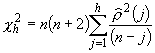
where n is the number of residuals

and  is the sample autocorrelation of the residuals at lag .

The null hypothesis that the residuals are independent and normally distributed is rejected with significance a if the calculated statistic exceeds the  quantile of the chi-squared distribution with h degrees of freedom.  In practice the Ljung-Box statistic is calculated out to lag 20 (h = 20).

 

ARIMA: Externally Validate the Model

The fitted model should now be applied to a sample of data from the modeled series that were not used to estimate the parameters.  This is usually done by holding out a portion of the available data or by using a second sample separated in time from the one used to develop the model.  Goodness of fit measures can be compared to the results achieved on the model development data.  Although one would expect the fit to be better to the development data, the performance should not be markedly worse for the model evaluation data.

An often-overlooked step in model validation is to compare forecasts from the fitted model to naïve or heuristic forecasts.  For a stationary series (no differencing required), a reasonable naïve forecast to compare to would be .  For a first difference series (a first ordinary difference required for stationarity), one might compare the fitted model forecasts to .  Similar non-fitted heuristic forecasts can be developed for seasonal series as well.  If the fitted model cannot consistently outperform heuristic forecasts on the model evaluation data, then its usefulness is questionable.  Paired samples statistical tests such as the Wilcoxon Signed-Rank test can be used to assess the statistical significance of differences in performance based on absolute deviation or absolute percentage error.

 

ARIMA: Document the Model

The validated model should be thoroughly documented.  All assumptions should be clearly spelled out along with the rationale for any modeling decisions along the way.  Specific items to be documented include:

·         how outliers were handled

·         how stationarity was achieved

·         how the model parameters were estimated

·         the methodology and results of the analysis of the residuals

·         the methodology and results of model validation

ARIMA: Implement the Model

Fitted ARIMA models provide equations that can be used to calculate recursive forecasts.  For forecasting, past innovations are estimated by the forecast residual.  All future innovations are estimated as zero.

The best way to illustrate ARIMA forecasting is by example.  Say we have a fitted model for a 15 minute flow rates at a freeway counting station.  Furthermore, say that the model is an ARIMA (1,0,1)(0,1,1)₆₇₂ with parameters , , and .  If we denote the flow rate series as then the model in equation form:

Rewritten the equation becomes:

Estimating past innovations by model residuals, the one-step forecast equation becomes:

In other words, we now have a linear recursive forecast equation in terms of past observations and past residuals.

How is a time series model equation interpreted?

For exponential smoothing models, the fitted values for the smoothing parameters give a sense of the stability of the smoothed component.  The more stable the time series component the lower the associated smoothing parameter will be.  The closer a smoothing parameter is to zero, the closer the recursive smoothing is to a straight average of all observed values.  The closer a smoothing parameter is to one, the closer the recursive smoothing is to simply echoing back the most recent value.

ARIMA models need to be interpreted in light of the modeled process.  The fitted model should make some intuitive sense.  It is difficult to give general interpretations.

How is the variance estimate interpreted?

The error variance gives evidence about the magnitude of the random component in the process.  The higher the magnitude of the variance estimate is relative to the magnitude of observed values, the more dominated the process is by the stochastic component versus the deterministic component.

How are prediction intervals interpreted?

Stated simply, the forecaster has (1-a)% confident that an individual observation would falls within the prediction interval.

How are information criteria interpreted?

Information criteria can only be used to compare models on the same sample with the same number of residuals.  The criteria values have no absolute meaning.  When comparing two models, the one with the lowest information criterion value should perform better in forecasting for future samples of the modeled process.  Higher values either indicate poorer fit or too many parameters.

Are there ARIMA equivalents to exponential smoothing models?

Yes.  Simple exponential smoothing is equivalent to ARIMA (0,1,1).  Double exponential smoothing is equivalent to ARIMA (0,2,2).  Additive Holt-Winters smoothing is equivalent to the following ARIMA model:

           

            where the  is of the order S+1 with coefficients given by

           

            (Yar and Chatfield, 1990).

 

What methods can be used to detect and model outliers?

If the analyst believes that the presence of outliers is introducing bias in the model estimation, there are available techniques to detect and model the outliers.  The most extensive work has been done by Chen et al. (Chang, Tiao and Chen, 1988), (Chen and Liu, 1993a), and (Chen and Liu, 1993b).  The methods they have developed are based on a one-at-a-time search and model strategy.  The only software package that includes systematic outlier detection is based on their work but not widely used, namely the time series software distributed by Scientific Computing Associates.  This is definitely an area where more research is needed and the available software tools need to be improved.

What if the errors are not white noise?

If the residuals for the “best” model exhibit significant correlation, there may be a problem with model specification.  However, white noise residuals in a univariate model should not be pursued if they can only be achieved by adding parameters that are not supported by information criterion analysis.  The presence of clustered outliers could result in correlation in the residuals.  It may also be possible that a univariate model alone is insufficient to properly model the series in question.

 

 

Survival and hazard models are used to model the effect of time on the “failure” of an event, process, or condition, as well as the effect of other covariates.

1)                   Unambiguous time origin,

2)                   Scale for measuring the passage of time,

3)                   Unambiguous definition of failure,

4)                   A set of predictors (independent variables) thought to affect the failure process.

Continuous variable Y measured on a time scale,

Sample of observations on Y for vector of explanatory variables, X.

Goodness of fit statistics of observed time-to-failure data to various assumed failure distributions

Estimated effects of covariates, X, on time to failure

There are numerous characteristics of the modeling of survival data that warrant mention here. Note that modeling survival data is not covered in detail in this manuscript, and only some of the main highlights are provided. The references provided at the end of this chapter should be consulted for estimating survival models.

1)                   Censoring is a characteristic of survival data. In other words, there are experimental units observed over time period T that have ‘failed’ (e.g. died, crashed, recovered from illness, etc.), and the remaining experimental units have yet to fail because time has been censored, due to the end of the data collection period.

2)                   Often observed in survival data are time-dependent covariates. These are independent variables that vary over time for an individual or experimental unit, reflecting the changing status of an individual or unit over the duration of the study.

3)                   Central to the modeling of survival times is the notion of hazard and survival functions. A hazard function is a mathematical function that expresses the fraction of the population failing by time t. The survivor function, related to the hazard function, is the fraction still surviving at time t.

4)                   There are numerous probability functions that can serve as survival functions, such as exponential, gamma, Weibull, compound exponential, log logistic, extreme value distribution, and proportional hazards family of distributions.

5)                   Similar to other statistical models, there are components of variance (unexplained deviations from the survivor and hazard functions), and covariates that are thought to affect the survival time of experimental units.

6)                   Similar to other statistical models, models can be compared to determine: which covariates are thought to influence the survival process, and which probability distribution best approximates the survival process.

Cox, D.R. , and Oakes, D. Analysis of Survival Data. Chapman & Hall/CRC. New York, New York.

 

Greene, William, (1990).  Econometric Analysis.  Macmillan Publishing Company. Hillsdale, NJ.

 

McCullagh, P. and J.A. Nelder, (1983). Generalized Linear Models. Second Edition. Chapman and Hall, New York, New York.

 

Lee, Elisa T., (1992). Statistical Methods for Survival Data Analysis. John Wiley and Sons. New York.