Chapter
6
Nonparametric methods are uniquely useful for testing
nominal (categorical) and ordinal (ordered) scaled data--situations where parametric tests are not generally available. An important second use is when an underlying assumption for a
parametric method has been violated.
In this case, the interval/ratio scale data can be easily transformed
into ordinal scale data and the counterpart
nonparametric method can be used.
Inferential and
Descriptive Statistics: The nonparametric methods described in this chapter
are used for both inferential and descriptive statistics. Inferential statistics use data
to draw inferences (i.e., derive conclusions) or to make predictions. In this chapter, nonparametric inferential statistical methods are used to
draw conclusions about one or more populations from which the data samples have
been taken. Descriptive statistics aren’t used to make
predictions but to describe the data.
This is often best done using graphical methods.
Examples:
An analyst or engineer might be interested to assess the evidence regarding:
1. The difference between the
mean/median accident rates of several marked and unmarked crosswalks (when
parametric Student’s t test is invalid because sample distributions are not normal).
2. The differences between the absolute
average errors between two types
of models for forecasting traffic flow (when analysis of variance is invalid because
distribution of errors is not normal).
3. The relationship between the
airport site evaluation ordinal rankings of two sets of judges, i.e., citizens
and airport professionals.
4. The differences between
neighborhood districts in their use of a regional mall for purposes of planning
transit routes.
5. The comparison of accidents before
and during roadway construction to investigate if factors such as roadway
grade, day of week, weather, etc. have an impact on the differences.
6. The association between ordinal variables, e.g., area type and
speed limit, to eliminate intercorrelated dependent variables for estimating
models that predict the number of utility pole accidents.
7. The relative goodness of fit of possible
predictive models to the observed data for expected accident rates for
rail-highway crossings.
8. The relative goodness of fit of hypothetical
probability distributions, e.g., lognormal and Weibull, to actual air quality
data with the intent of using the distributions to predict the number of days
with observed ozone and carbon monoxide concentrations exceeds National Ambient
Air Quality Standards.
Nonparametric methods are contrasted to those that are
parametric. A generally accepted
description of a parametric method is one that makes specific assumptions with
regard to one or more of the population
parameters that characterize the underlying distribution(s) for which the test
is employed. In other words, it a test
that assumes the population distribution
has a particular form (e.g., a normal distribution) and involves hypotheses
about population
parameters. Nonparametric tests do not
make these kinds of assumptions about the underlying distribution(s) (but some
assumptions are made and must be understood).
Nonparametric methods use approximate solutions to
exact problems, while parametric methods use exact solutions to approximate
problems.
W.J. Conover
Remember the overarching purpose for employing a
statistical test is to provide a means for measuring the amount of subjectivity
that goes into a researcher’s conclusions.
This is done by setting up a theoretical model for an experiment.
Laws of probability are applied to this model to determine what the chances (probabilities) are for
the various outcomes of the experiment assuming chance alone determines the outcome of the experiment. Thus, the researcher has an objective basis
to decide if the actual outcome from his or her experiment were the results of the treatments applied or if
they could have occurred just as easily by chance alone, i.e., with no
treatment at all.
When the researcher has described an appropriate
theoretical model for the
experiment (often not a trivial task), the next task is to find the
probabilities associated with the model.
Many reasonable models have been developed for which no probability
solutions have ever been found. To
overcome this, statisticians often change a model slightly in order to be able
to solve the probabilities with the hope that the change doesn’t render the model unrealistic. These changes
are usually “slight” to try to minimize the impacts, if possible. Thus, statisticians can obtain exact
solutions for these “approximate problems.”
This body of statistics
is called parametric statistics and
includes such well-known tests as the “t
test” (using the t distribution) and
the F test (using the F distribution) as well as others.
Nonparametric testing takes a different approach, which
involves making few, if any, changes in the model itself. Because the exact probabilities can’t be
determined for the model, simpler, less sophisticated methods are used to find
the probabilities--or at least a good approximation of the probabilities. Thus,
nonparametric methods use approximate solutions to exact problems, while
parametric methods use exact solutions to approximate problems.
Statisticians disagree about which methods are parametric
and which are nonparametric. Such
disagreements are beyond the scope of this discussion. Perhaps one of the easiest definitions to
understand, as well as being fairly broad, is one proposed by W.J. Conover
(1999, p.118).
Definition: A statistical method is nonparametric if it
satisfies at least one of the following criteria:
1. The method may be used on data with a nominal scale of
measurement.
2.
The method may be used on data with an ordinal scale of
measurement.
3.
The method may be used on data
with an interval or ratio scale of measurement, where the distribution function of the random
variable producing the data are unspecified (or specified except for an
infinite number of unknown parameters
Herein lies a primary usefulness
of nonparametric tests: for testing nominal and ordinal scale data.
There is debate about using nonparametric tests on interval and ratio scale data. There is general agreement among researchers
that if there is no reason to believe that one or more of the assumptions of a
parametric test has been violated, then the appropriate parametric test should
be used to evaluate the data. However,
if one or more of the assumptions have been violated, then some (but not all)
statisticians advocate transforming the data into a format that is compatible with the appropriate
nonparametric test. This is based on
the understanding that parametric tests generally provide a more powerful test
of an alternative hypothesis
than their nonparametric counterparts; but if one or more of the underlying
parametric test assumptions is violated, the power advantage may be negated.
The researcher should not spend too much time worrying
about which test to use for a specific experiment. In almost all cases, both tests applied to the same data will lead to identical or
similar conclusions. If conflicting results occur, the researcher would be well
advised to conduct additional experiments to arrive at a conclusion, rather
than simply pick one or the other method as being “correct.”
Environment
Chock, David P. and Paul S. Sluchak. (1986). Estimating
Extreme Values of Air Quality Data
Using Different Fitted Distributions.
Atmospheric Environment, V.20, N.5, pp. 989-993. Pergamon Press
Ltd. (Kolmogorov-Smirnov Type Goodness
of Fit (GOF) Tests and Chi-Square GOF Test)
Safety
Ardeshir, Faghri, Demetsky Michael J. (1987). Comparison
of Formulae for Predicting Rail-Highway Crossing Hazards. Transportation Research Record
#1114 pp. 152-155. National Academy of Sciences. (Chi-Square Goodness of Fit Test)
Davis, Gary A. and Yihong Gao. (1993). Statistical
Methods to Support Induced Exposure Analyses of Traffic Accident Data. Transportation Research Record
#1401 pp. 43-49. National Academy of Sciences.
(Chi-Square Test for Independence)
Gibby, A. Reed, Janice Stites, Glen S. Thurgood, and Thomas
C. Ferrara. (1994). Evaluation of Marked and Unmarked Crosswalks at
Intersections in California. Federal Highway Administration,
FHWA/CA/TO-94-1 and California Department of Transportation (Caltrans) CPWS 94-02, 66 pages. (Mann-Whitney
Test for Two Independent Samples)
Hall,
J. W. and V. M. Lorenz.(1989). Characteristics of Construction-Zone
Accidents. Transportation
Research Record #1230 pp. 20-27. National Academy of Sciences. (Chi-Square
Test for Independence)
Kullback, S. and John C. Keegel. (1985). Red Turn Arrow:
An Information-Theoretic Evaluation. Journal of Transportation Engineering, V.111, N.4, July, pp. 441-452.
American Society of Civil Engineers. (Inappropriate use of Chi-Square Test for
Independence)
Zegeer, Charles V., and Martin R. Parker Jr. (1984). Effect
of Traffic and Roadway Features on Utility Pole Accidents. Transportation Research Record
#970 pp. 65-76. National Academy of Sciences.
(Kendall’s Tau Measure of Association for Ordinal Data)
Traffic
Smith, Brian L. and Michael J. Demetsky. (1997). Traffic
Flow Forecasting: Comparison of Modeling Approaches. Journal of Transportation Engineering, V.123,
N.4, July/August, pp. 261-266. American Society of Civil Engineering. (Wilcoxon
Matched-Pairs Signed-Ranks Test for Two Dependent Samples)
Transit
Ross, Thomas J. and Eugene M. Wilson. (1977). Activity
Based Transit Routing. Transportation
Engineering Journal, V.103,
N.TE5, September, pp. 565-573. American Society of Civil Engineers. (Chi-Square
Test for Independence)
Planning
Jarvis, John J., V. Ed Unger, Charles C. Schimpeler, and
Joseph C. Corradino. (1976). Multiple Criteria Theory and Airport Site
Evaluation. Journal of Urban Planning and Development Division, V.102, N.UP1, August, pp.
187-197. American Society of Civil
Engineers. (Kendall’s Tau Measure of Association
for Ordinal Data)
·
W. J. Conover.
“Practical Nonparametric Statistics.”
Third Edition, John Wiley & Sons, New York, 1999.
·
W. J. Conover.
“Practical Nonparametric Statistics.”
Second Edition, John Wiley & Sons, New York, 1980.
·
Richard A. Johnson.
“Miller & Freund’s Probability and Statistics For Engineers.”
Prentice Hall, Englewood Cliffs, New Jersey, 1994.
·
Douglas C. Montgomery.
“Design and Analysis of Experiments.”
Fourth Edition, John Wiley & Sons, New York, 1997.
·
David J. Sheskin.
“Handbook of Parametric and Nonparametric Statistical Procedures.” CRC Press, New York, 1997.
Graphical methods can be thought of as a way to obtain a
“first look” at a group of data. It
does not provide a definitive interpretation of the data, but can lead to an
intuitive “feel” for the data. However,
this “first look” can be deceiving because the human mind wants to classify
everything it views based on something it already knows. This can lead to an erroneous first
impression that can be hard for a researcher to dismiss; even as evidence
mounts that it may be wrong. This is
human nature at work, wanting to be consistent. It is important for a researcher to be aware of this need for
consistency, which can cloud objectivity.
The parable of the three blind men encountering an
elephant for the first time effectively illustrates this human tendency to make
a judgement based on past experience and then to “stop looking” for more
clues. In the parable, the three blind
men approached the elephant together.
The first man touches the elephant’s trunk and thoroughly investigates
it. He backs away and declares “the
elephant is exactly like a hollow log, only alive and more flexible.” The second man touches one of the elephant’s
massive feet and explores it in many places.
He backs away and declares, “the elephant is very much like a large tree
growing from the ground, only its bark is warm to the touch.” The last man grasps the elephant’s tail and
immediately declares “the elephant is simply a snake that hangs from something,
probably a tree.”
All of the information gathered by the three blind men is
important and pooled might provide a “good” model of an elephant.
Graphical methods should be thought of as a single blind investigation.
The data viewed is not
wrong, but a conclusion drawn solely from them can be wrong. Keep in mind that the purpose of graphical
methods is simply to get a first look at the data without drawing conclusions. It can, however, lead to hypotheses that guide further
investigation.
Examples:
An analyst or engineer might be interested in exploring data to:
1. See if potential relationships,
either linear or curvilinear, exist between a variable of interest whose values may depend on several
other variables.
2. See if interactions (relationships)
may exist between a variable
and two other variables.
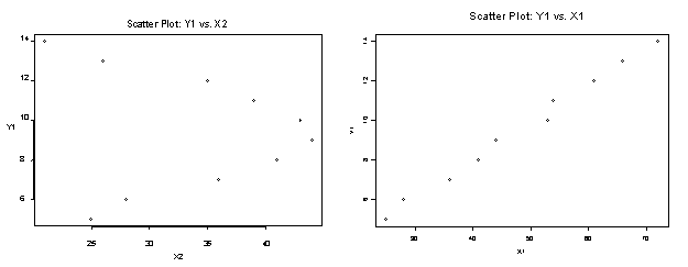
Scatter plots are the workhorses of graphical
methods. In two dimensions, the data points are simply plotted by
specifying two variables to form the axes.
This technique is often used to develop a first impression about the
relationship between two variables. For
example, the variables in the two scatter plots below appear to have quite
different relationships.
As a first look, X1 appears to have a linear relationship
with Y1 while X2 appears to have a non-linear relationship. Hypothesizing such apparent relationships
are useful in selecting a preliminary model type and relationship. Many statistical software packages make it easy for the user to
study such relationships among all the variables in the data. This method is typically called “pairwise”
scatter plots but other terms are also used.
The three variables explored in the previous scatter plots are used
again to plot the pairwise scatter plots shown below.
Figure 17: Scatter Plots of Y1 vs. X1, and Y1 vs. X2
By using pairwise scatter plots, the relationships among
all the variables may be explored with a single plot. However, as the number of variables increases, using a single
plot reduces the individual plots too small to be useful. In this case, the variables can be plotted
in subsets.
Figure 18: Pair-wise Scatter Plots for Y1, X2, and X2
The scatter plots described so far are
two-dimensional. Three-dimensional
methods are also available and are often used in exploring three variables from
the data. The data displayed in this fashion form as a “point cloud”
using three axes. The more powerful
statistical software packages allow these point clouds to be rotated or spun
around any axis. This gives hints as to
any interactions between two variables as it affects a third variable. Another feature often available is a brush
technique, which allows the user to select specific points to examine. These points then become bigger or of a
different color than the remainder of the data, which allows the user to see
their spatial relationship within the point cloud. Usually a pairwise scatter plot is simultaneously displayed on
the same screen and the selected points are also highlighted in each of these
scatter plots. This allows the user to
study individual points or clusters of points.
Examples that are useful to explore are outliers and clusters of points that are seemingly isolated
from the rest of the data
points.
Three-dimensional graphics allow the user to investigate
three variables simultaneously. Two
plots that are often used are the contour plot and the surface plot. Examples using the three variables explored
previously in the scatter plots are shown below. The contour plot shows the isobars of Y1 for the range of values of X1 and X2
contained within the plot. The surface
plot fits a “wire mesh” through the X1, X2, and Y1 coordinates to give the user
a perspective of the surface created by the data. In both of these graphs the values between the data values are interpolated. The user is cautioned that these
interpolations are not validated and a “smooth” transition from one point to
the next may not be a true representation of the data. Like all graphical methods, these should be
used only to obtain a first look at the data, and when appropriate, aid in
developing preliminary hypotheses--along with other available information--for
modeling the data.
Figure 19: Contour and Surface Plots for Variables Y1, X1, and X2
One way to better understand what descriptive statistics are is to
first describe inferential statistics.
If the data being
investigated are a sample that
is representative of a larger population, important conclusions about that population can often be inferred
from analysis of the sample. This is
usually called inferential statistics, although sometimes it may be called
interpretative statistics. Because such
inferences cannot be absolutely certain, probability is used in stating
conclusions. This is an inductive
process and is used in the sections of this chapter that follow this one.
Descriptive techniques are discussed in this section and
are another important first step in exploring data. The purpose of these techniques is to describe and analyze a sample
without drawing any conclusions or inferences about a larger group from which
it may have been drawn. This is a deductive process and is quite useful in
developing an understanding of the data.
Occasionally this is all that is needed, but often it is a preliminary
step toward modeling the data.
Examples:
An analyst or engineer might be interested in exploring data to:
1. Quantitatively assess its
dispersion, i.e., to determine whether ifs values are bunched tightly about
some central value or not.
2. Quantitatively assess all the
values of the data, perhaps to qualitatively examine a suspicion that the data may have some distribution of
values that is similar to something the investigator has seen before.
3. Quantitatively compare two or more
sets of data in order to
qualitatively examine what potential similarities or significant differences
might be present.
Almost all general statistical reference books and
textbooks thoroughly describe these types of descriptive statistics, one such
reference is Johnson (1994). Briefly
the mean is typically the arithmetic
mean, which is simply the average
of all the numbers in the data
sample. The median is the middle value when all the values in a data variable are ranked in order
such that ties are ranked one above the other rather than together. The median is also the second quartile of the data
variable. Quartiles are the dividing
points that separate the data
variable values into four equal parts.
The first or lower quartile has 1/4 or 25% of the ranked data variable values below its
value. The third or upper quartile has
3/4 or 75% of the values below it. Some
references reverse the first and third labels, so the upper and lower labels
create less confusion.
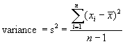
The variance
and standard deviation are quantitative measures of dispersion, i.e., the
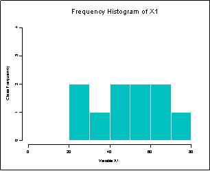
spread of a distribution. Histograms
and Boxplots are graphical ways to view the dispersion. A frequency distribution
is simply a table that divides a set of observed data values into a suitable number of classes or
categories, indicating the number of items belonging in each class. This provides a useful summary of the
location, shape and spread of the data
values. Consider the data used in the previous examples,
which are provided in the following table.
Table 4: Observed Data Values
|
Y1
|
X1
|
X2
|
|
5
|
25
|
25
|
|
6
|
28
|
28
|
|
7
|
36
|
36
|
|
8
|
41
|
41
|
|
9
|
44
|
44
|
|
10
|
53
|
43
|
|
11
|
54
|
39
|
|
12
|
61
|
35
|
|
13
|
66
|
26
|
|
14
|
72
|
21
|
In order to create a frequency
distribution for a variable,
appropriate classes must be selected for it.
Using both X1 and X2 as examples, classes of 0 to 10, 11 to 20, etc. are
chosen and a frequency table
constructed as shown below.
Table 5: Frequency Distribution of Observed Data
|
Class
Limits
|
X1
|
X2
|
|
0 - 10
|
0
|
0
|
|
11-20
|
0
|
0
|
|
21-30
|
2
|
4
|
|
31-40
|
1
|
3
|
|
41-50
|
2
|
3
|
|
51-60
|
2
|
0
|
|
61-70
|
2
|
0
|
|
71-80
|
1
|
0
|
|
Totals
|
10
|
10
|
|
Variance
|
252.00
|
67.73
|
|
Standard Deviation
|
15.87
|
8.23
|
The variance
and standard deviation are also shown in the table along with the frequency
distribution. These are measures of the
spread of the data about the
mean. If all the values are bunched
close to the mean, then the spread is “small.”
Likewise, the spread is large if all the values are scattered widely
about their mean. A measure of the spread of data is useful to supplement the mean in describing the data. If a set of numbers x1,
x2, ... , xn has a mean xbar,
the differences x1- xbar,
x2- xbar,..., xn- xbar are
called the deviations from the
mean. Because the sum of these
deviations is always zero, an alternative approach is to square each deviation.
The sample variance, s2, is essentially the average of the squared deviations
from the mean.
By dividing the sum of squares by its degrees of freedom, n-1,
an unbiased estimate of the population
variance is obtained. Notice
that s2 has the wrong
units, i.e., not the same units as the variable itself. To
correct this, the standard deviation
is defined as the square root of the variance, which has the same units as the
data. Unlike the variance
estimate, the estimated standard deviation is biased, where the bias becomes
larger as sample sized become smaller.
.
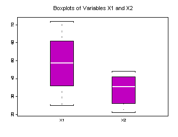
Figure 20: Frequency Histograms of X1 and X2
While these quantitative descriptive statistics are useful, it is often valuable to
provide graphical representations of them.
The frequency distributions can be shown graphically using frequency histograms as shown
below for X1 and X2.
As can be seen from these two frequency histograms, X2 has a much smaller spread
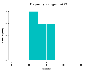
(standard deviation = 8.23) than does X1 (standard deviation = 15.87). Another plot, the boxplot, also shows the
quartiles of the frequency. These are
shown in Figure 21 for X1 and X2.
Different statistical software packages typically depict
Boxplots in different ways, but the one shown here is typical. Boxplots are particularly effective when
several are placed side-by-side for comparison. The shaded area indicates the middle half of the data. The center line inside this shaded area is
drawn at the median value. The upper edge of the shaded area is the
value of the upper quartile and the lower edge is the value of the lower
quartile. Lines extend from the shaded
areas to the maximum and minimum values of the data indicated by horizontal lines.
Figure 21: Boxplots of X1 and X2
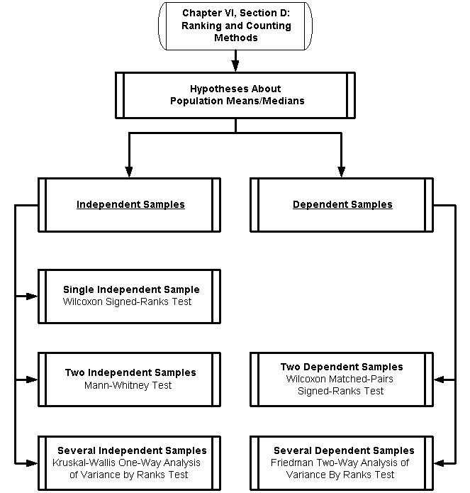
The primary purpose of ranking and counting methods is hypothesis testing for ordinal
scale data and for interval and ratio scale data without reliance on
distribution assumptions. Data may be
nonnumeric or numeric. If the data are
nonnumeric but ranked as in ordinal-type data (e.g., low, medium, high), the methods in this section
are often the most powerful ones available (Conover, 1999). These methods are valid for continuous and
discrete populations as well as mixtures of the two.
The hypotheses tested using these methods all involve
medians. While at first glance this may
seem to be of limited usefulness, it is surprisingly versatile. When the distributions of the random
variables tested are assumed to be symmetric, the mean and the median are equal so these hypotheses also test
means. Usually the data, or statistics extracted from the
data, are ranked from least to greatest.
Data may have many ties. Two
observations are said to be tied if they have the same value.
Early results in nonparametric statistics required the assumption of a continuous random variable in order for the
tests based on ranks to be valid.
Research results reported by Conover (1999) and others have shown that
the continuity assumption is not necessary.
It can be replaced by the trivial assumption that P(X = x) < 1 for each x.
It is unlikely that any sample
will be taken from a population
with only a single member. Since this
assumption is trivial, it is not listed for each test in this section, but it
is what allows these tests to be valid for all types of populations:
continuous, discrete, or mixtures of the two.
Examples:
An analyst or engineer might be interested to assess the evidence regarding the
difference between the mean/median values of:
1. Accident rates of several marked
and unmarked crosswalks (when parametric Student’s t test is invalid because sample distributions are not
normal).
2. The differences between the
absolute average errors between
two types of models for forecasting traffic flow (when analysis of variance is invalid because
distribution of errors is not normal).
Data collection is usually called sampling in statistical
terms. Sampling is the process of
selecting some part of a population
to observe so as to estimate something of interest about the whole
population. A population is the statistical term
referring to the entire aggregate of individuals, items, measurements, things,
numbers, etc. from which samples are drawn.
Two samples are said to be mutually independent if each sample is comprised of different
subjects. Dependent samples usually
have the same subjects as in a comparative study, e.g., a before and after
study or how a subject responds to two different situations (called treatments).
Hypotheses About
Population Medians for Independent Samples
This rank test was devised by F. Wilcoxon in 1945. It is designed to test whether a particular sample came from a population with a specified
median. This test is similar to but
more powerful than the classic sign test, which is not presented here. The classic sign test is the oldest of all
nonparametric tests, dating back to 1710, when it was used by J. Arbuthnott to
compare the number of males born in London to the number of females born
there. The sign test is simpler to use
than the more powerful nonparametric tests and is popular for that reason. With today’s computer software packages,
however, this is no longer a factor.
1) The
sample is a random sample.
2) The
measurement scale is at least interval.
3) The
underlying population
distribution is symmetrical. A distribution of a random variable X is symmetrical about a line having a
value of x = c if the probability of the variable being on one side of the line is equal to the
probability of it being on the other side of the line, for all values of the
random variable. Even when the analyst
may not know the exact distribution of a random variable, it is often
reasonable to assume that the distribution
is symmetric. This assumption is not as
rigid as assuming that the distribution
is normal. If the distribution is symmetric, the mean coincides with the median
because both are located exactly in the middle of the distribution, at the line
of symmetry. Therefore, the benefit of adding this symmetry
assumption is that inferences concerning the median are also valid statements for the mean. The liability of adding this assumption is
that the required scale of measurement is increased from ordinal to interval.
The data
consist of a single random sample X1,
X2, ... , Xn of size n that has a median m.
Wilcoxon Signed-Ranks Test is used to test whether a
single random sample of size n, X1,
X2, ... , Xn comes from a population in which the median
value is some known value m.
A. Two-sided test
Ho: The
median of X equals m.
Ha:
The median of X is not m.
B. Upper-sided test
Ho: The
median of X is £ m.
Ha:
The median of X is > m.
C. Lower-sided test
Ho: The
median of X is ³ m.
Ha:
The median of X is < m.
Note that the mean
may be substituted for the median in these hypotheses because of the assumption
of symmetry of the distribution of X.
The ranking for this test is not done on the observations
themselves, but on the absolute values of the differences between the
observations and the value of the median
to be tested.

All differences of zero are omitted. Let the number of pairs remaining be denoted
by n’, n’ < n. Ranks from 1 to n’ are assigned to the n’
differences. The smallest absolute
difference |Di | is ranked
1, the second smallest |Di |
is ranked 2, and so forth. The largest
absolute difference is ranked n’. If groups of absolute differences are equal
to each other, assign a rank to each equal to the average of the ranks they would have otherwise been
assigned. For example, if four absolute
differences are equal and would hold ranks 8, 9, 10, and 11, each is assigned
the rank of 9.5, which is the average
of 8, 9, 10, and 11.
Although the absolute difference is used to obtain the
rankings, the sign of Di
is still used in the test statistic.
Ri, called the
signed rank, is defined as follows:
Ri = the rank assigned to |Di | if Di is positive.
Ri = the negative of the rank assigned to |Di | if Di is negative.
The test statistic
T+ is the sum of the
positive signed ranks when there are no ties and n’ < 50. Lower quantiles
of the exact distribution of T+ are given in Table C-8. Under the null hypothesis that the Di s have mean 0.

Based on the relationship that the sum of the absolute
differences is equal to n’ (n’ + 1) divided by 2, the upper
quantiles wp are found by the relationship

If there are many ties, or if n’ > 50, the normal approximation test statistic T is used which uses all of the signed ranks, with their + and -
signs. Quantiles of the approximate distribution of T are given in a Normal Distribution Table.

For the two-sided test, reject the null hypothesis Ho at level a
if T+ (or T) is less than its a/2
quantile or greater than its 1 - a/2
quantile from Table C-8 for T+
(or the normal distribution, see Table C-1 for T). Otherwise, accept Ho (meaning the median (or mean) of X equals m).
For the upper-tailed test, reject the null hypothesis Ho at level a
if T+ (or T) is greater than its a
quantile from Table C-8 for T+
(or the Normal Table C-1 for T). Otherwise, accept Ho (meaning the median (or mean) of X
is less than or equal to m). The p-value,
approximated from the normal distribution, can be found by

For the lower-tailed test, reject the null hypothesis Ho at level a
if T+ (or T) is less than its a quantile
from Table C-8 for T+ (or
the Normal Table C-1 for T). Otherwise, accept Ho (meaning the median (or mean) of X
is greater than or equal to m). The p-value,
approximated from the normal distribution, can be found by

The two-tailed p-value
is twice the smaller of the one-tailed p-values
calculated above.
Computational
Example: (Adapted from Conover
(1999, p. 356-357)) Thirty observations on the random variable X
are measured in order to test the hypothesis
that E (X), the mean of X, is no smaller than 30 (lower-tailed test).
Ho: E
(X) (the mean) ³ m.
Ha: E
(X) (the mean) < m.
The observations, the differences, Di = (Xi - m), and the ranks of the
absolute differences |Di |
are listed below. The thirty
observations were ordered first for convenience.
Table 6: Ranking Statistics on 30 Observations of X
|
Xi
|
Di = (Xi
- 30)
|
Rank of |Di |
|
|
Xi
|
Di = (Xi
- 30)
|
Rank of |Di |
|
|
23.8
|
-6.2
|
17
|
|
35.9
|
+5.9
|
15*
|
|
26.0
|
-4.0
|
11
|
|
36.1
|
+6.1
|
16*
|
|
26.9
|
-3.1
|
8
|
|
36.4
|
+6.4
|
18*
|
|
27.4
|
-2.6
|
6
|
|
36.6
|
+6.6
|
19*
|
|
28.0
|
-2.0
|
5
|
|
37.2
|
+7.2
|
20*
|
|
30.3
|
+0.3*
|
1
|
|
37.3
|
+7.3
|
21*
|
|
30.7
|
+0.7*
|
2
|
|
37.9
|
+7.9
|
22*
|
|
31.2
|
+1.2*
|
3
|
|
38.2
|
+8.2
|
23*
|
|
31.3
|
+1.3*
|
4
|
|
39.6
|
+9.6
|
24*
|
|
32.8
|
+2.8*
|
7
|
|
40.6
|
+10.6
|
25*
|
|
33.2
|
+3.2*
|
9
|
|
41.1
|
+11.1
|
26*
|
|
33.9
|
+3.9*
|
10
|
|
42.3
|
+12.3
|
27*
|
|
34.3
|
+4.3*
|
12
|
|
42.8
|
+12.8
|
28*
|
|
34.9
|
+4.9*
|
13
|
|
44.0
|
+14.0
|
29*
|
|
35.0
|
+5.0*
|
14
|
|
45.8
|
+15.8
|
30*
|
There are no ties in the data nor is the sample size greater than 50. Therefore, from Table C-8, Quantiles of Wilcoxon Signed Ranks
Test Statistic, for n’ = 30, the 0.05
quantile is 152. The critical region of size £ 0.05 corresponds to values of the test statistic less than 152. The test statistic T+
= 418. This is the sum of all the
Ranks, which have positive differences, as noted in the table by
asterisks. Since T+ is not within the critical region, Ho is accepted, and the analyst concludes that the mean of X is greater than 30.
The approximate p-value
is calculated by the following equation.
Recall that the summation of the squares of a set of numbers from 1 to N
is equal to [N (N+1) (2N + 1) / 6].

The normal distribution
table shows that the p-value is
greater than 0.999 when the mean is no smaller than 30, i.e., there is a
probability greater than 99.9% that the mean is greater than or equal to 30.
The Mann-Whitney test, sometimes referred to as the
Mann-Whitney U test, is also called
the Wilcoxon test. There are actually
two versions of the test that were independently developed by Mann and Whitney
in 1947 and Wilcoxon in 1949. They employ
different equations and use different tables, but yield comparable
results. One typical situation for
using this test is when the researcher wants to test if two samples have been
drawn from different populations.
Another typical situation is when one sample was drawn, randomly divided into two sub-samples,
and then each sub-sample receives a different treatment.
The Mann-Whitney test is often used instead of the t-test for two independent samples when
the assumptions for the t-test may be
violated, either the normality assumption or the homogeneity of variance
assumption. If a distribution function is not a
normal distribution function, the probability theory is usually not available
when the test statistic is
based on actual data. By contrast, the
probability theory based on ranks, as used here, is relatively simple. Additionally, according to Conover (1999),
comparisons of the relative efficiency between the Mann-Whitney test and the
two-sample t-test is never too bad
while the reverse is not true. Thus the Mann-Whitney test is the safer test to
use.
One can intuitively understand the statistics involved in this
test. First combine the two samples
into a single sample and order
them. Then rank the combined sample
without regard to which sample
each value came from. A test statistic could be the sum of the
ranks assigned to one of the samples.
If the sum is too small or too great, this gives an indication that the
values from its population tend
to smaller or larger than the values from the other sample. Therefore, the null hypothesis that there is no
difference between the two populations can be rejected, if the ranks of one
sample tend to be larger than the ranks of the other sample.
1) Each
sample is a random sample from
the population it represents.
2) The
two samples are independent of each other.
3) If
there is a difference in the two population
distribution functions F (x) and G (y), it is a difference
in the location of the distributions.
In other words, if F (x) is not identical with G (y),
then F (x) is identical with G (y + c),
where c is some constant.
4) The
measurement scale is at least ordinal.
Let X1,
X2, . . . , Xn represent a random sample of size n from population 1 and let Y1,
Y2, . . . , Ym represent a random sample of size m from population 2. Let n + m = N. Assign ranks 1 to N to all the observations from smallest
to largest, without regard from which population they came from.
Let R (Xi) and R (Yj) represent the ranks
assigned to Xi and Yj for all i and j. If several values are
tied, assign each the average of
the ranks that would have been assigned to them had there been no ties.
The Mann-Whitney test is unbiased and consistent when the four listed
assumptions are met. The inclusion of
assumption 3 allows the hypotheses to be stated in terms of the means. The expected value E (X) is the mean.
A. Two-sided test
Ho: E
(X) = E (Y)
Ha:
E (X) ¹ E (Y)
B. Upper-sided test
Ho: E
(X) ³ E (Y)
Ha:
E (X) < E (Y)
C. Lower-sided test
Ho: E
(X) £ E (Y)
Ha:
E (X) > E (Y)
The hypotheses shown here are for testing means. Different hypotheses are also discussed in
most texts (e.g., Conover (1999) and Sheskin (1997)) that test to see if the
two samples come from identical distributions.
This does not require assumption 3.
Elsewhere in this chapter, the Kolmogorov-Smirnov type goodness-of-fit
tests are described which also test if two (or more) samples are drawn from the
same distribution. For this reason, the
identical distribution hypotheses
of the Mann-Whitney test are not discussed here.
The test statistic
T can be used when there are no ties
or few ties. It is simply the sum of
the ranks assigned to the sample
from population one.
If there are many ties, the test statistic T1 is obtained which
simply subtracts the mean from T and divides by the standard deviation
where SRi2 is the sum of the squares
of all N of the ranks or average ranks actually used in both
samples.
Lower quantiles wp-1
of the exact distribution of T are given for n and m values of 20 or
less in Table C-6. Upper quantiles wp
are found by the relationship
Perhaps more convenient is the use T’ which can be used with the lower quartiles in Table C-6 whenever
an upper-tail test is desired.
When there are many ties in the data, T1 is used which is approximately a standard normal random variable. Therefore, the quantiles for T1 are found in Table C-1,
which is the standard normal table.
When n or m is greater than 20 (and there are
still no ties), the approximate quantiles are found by the normal approximation
given by
for quantiles when n
or m is greater than 20, where zp is the pth quantile of a standard
normal random variable obtained from Table C-1.
For the two-sided test, reject the null hypothesis Ho at level a
if T (or T1) is less than its a/2 quantile or greater than its 1 - a/2
quantile from Table C-6 for T (or
from the Standard Normal Table C-1for T1). Otherwise, accept Ho if T (or T1) is between, or equal to
one of, the quantiles indicating the means of the two samples are equal.
For the upper-tailed test, large values of T indicate that H1 is true.
Reject the null hypothesis
Ho at level a if T (or T1) is greater than its a quantile from Table C-6 for T (or from the Standard Normal Table C-1 for T1). It may be
easier to find T’ = n (N+1)
- T and reject Ho if T’ is
less than its a from
Table C-6. Otherwise, accept Ho
if T (or T1) is less than or equal to its a quantile indicating the mean of
population 1 is less than or equal to the mean of population
2.
For the lower-tailed test, small values of T indicate that H1 is true.
Reject the null hypothesis
Ho at level a if T (or T1) is less than its a quantile from Table C-6 for T (or from the Standard Normal Table C-1 for T1). Otherwise,
accept Ho if T (or T1) is greater than or equal to its a
quantile indicating the mean of population 1 is greater than or equal to the mean of population 2. If
the n or m is larger than 20, use
When n or m is greater than 20 (and no ties), the
quantiles used in the above decisions are obtained directly from the equation
given previously for this condition.
Computational
Example: (Adapted from Conover
(1999, p. 278-279)) Nine pieces of flint were collected for a simple
experiment, four from region A and five from region B. Hardness was judged by rubbing two pieces of
flint together and observing how each was damaged. The one having the least damage was judged harder. Using this method all nine pieces of flint
were tested against each other, allowing them to be rank ordered from softest
(rank 1) to hardest (rank 9).
Table 7: Hardness of Flint Samples from Regions A and B
|
Region
|
Rank
|
|
A
|
1
|
|
A
|
2
|
|
A
|
3
|
|
B
|
4
|
|
A
|
5
|
|
B
|
6
|
|
B
|
7
|
|
B
|
8
|
|
B
|
9
|
The hypothesis
to be tested is
Ho: E
(X) = E (Y) or the flints from
regions A and B have the same means
Ha:
E (X) ¹ E (Y)
or the flints do not have the same mean
The Mann-Whitney two-sided test is used with n = 4 and m = 5. The test statistic T is calculated by
T = sum
of the ranks of flints from region A
T =
1 + 2 + 3 + 5 = 11
The two-sided critical region
of approximate size a =
0.05 corresponds to values of T less
than 12 and greater than 28, which is calculated by
Since the test statistic of 11 falls inside the lower critical region,
less than 12, the null hypothesis
Ho is rejected and the
alternate hypothesis is
accepted, i.e., the flints from the two regions have different harnesses. Because the direction of the difference, it
is further concluded that the flint in region A is softer than the flint in
region B.
Safety Example: In an
evaluation of marked and unmarked crosswalks (Gibby, Stites, Thurgood, and
Ferrara, Federal Highway Administration FHWACA/TO-94-1, 1994), researchers in
California investigated if marked crosswalks at intersections had a higher
accident frequency than
unmarked crosswalks. The data was analyzed in four major
subsets: (1) all intersections, (2) intersections with accidents, (3)
intersections with signals, and (4) intersections without signals. Each of these was further dived into (1)
intersections with crosswalks on the state highway approaches only and (2)
intersections with crosswalks on all approaches. This approach provided many subsets of data for analysis.
Two hypotheses were tested for each subset of data using a two-sided Mann-Whitney Test for two
independent samples:
Ho: There is no difference between accident rates on marked and
unmarked crosswalks.
Ha: There is a difference between the accident rates on marked and
unmarked crosswalks.
A 5% or less level of significance
was used as being statistically significant.
Several tests were made for each subset for which the researchers had
sufficient data. In some of the tests,
the sample size was greater
than 20 so the approximate quantiles were found by the normal
approximation. Where sample sizes were less than this,
the quantiles were calculated according to the appropriate formula that matched
the specific reference tables used by the researchers. From these numerous tests, they were able to
draw these general conclusions:
1. At unsignalized intersections
marked crosswalks clearly featured higher pedestrian-vehicle accident rates.
2. At signalized
intersections the results were inconclusive.
It should be noted that the names of many nonparametric test are not
standardized. In this study the researchers
refer to the test they used as a Wilcoxon Rank Sum Test. Their test is the same as that called the
Mann-Whitney Test for Two Independent Samples in this manual. Further, they used a different reference for
their test than cited here. This means they
used a slightly different form of the test statistic than used in this manual, which corresponded to
the tables in their reference versus the tables in the reference cited in this
manual. This example emphasizes the
care that must be taken when applying nonparametric tests regarding matching
the test statistic employed
with its specific referenced tables.
One should not, for example, use a test statistic from this manual with tables from some other
source.
Kruskal and Wallis (1952) extended the Mann-Whitney method
to be applicable to two or more independent samples. The typical situation is to test the null hypothesis that all medians of the
populations represented by k random
samples are identical against the alternative that at least two of the population medians are
different.
The experimental
design that is usually a precursor to applying this test is called the completely randomized design. This design allocates the treatments to the
experimental units purely on a chance basis.
The usual parametric method of analyzing such data is called a one-way
analysis of variance or sometimes is referred to as a single-factor between-subjects analysis of variance. This parametric method assumes normal
distributions in using the F test
analysis of variance on the
data. Where the normality assumption is
unjustified, the Kruskal-Wallis test can be used.
1. Each
sample is a random sample from
the population it represents.
2. All
of the samples are independent of each other.
3. If
there is a difference in any of the k population
distribution functions F (x1),
F (x2), ..., F (xk), it is a difference in
the location of the distributions. For
example, if F (x1) is not identical with F (x2), then F (x1)
is identical with F (x2 + c), where c is some
constant.
4. The
measurement scale is at least ordinal.
The data
consist of several random samples k
of possibly different sizes. Describe
the ith sample of size ni by Xi1, Xi2, . . . , Xini,
The data can be arranged
in k columns, each column containing
a sample denoted by Xi,j where i = 1 to k and j = 1 to ni for each i sample.
Table 8: Input Table for Kruskal-Wallis One-Way Analysis of
Variance
|
sample 1
|
sample 2
|
. . .
|
sample k
|
|
X1,1
|
X2,1
|
. . .
|
Xk,1
|
|
X1,2
|
X2,2
|
. . .
|
Xk,2
|
|
. . .
|
. . .
|
. . .
|
. . .
|
|
X1,n1
|
X2,n2
|
. . .
|
Xk,nk
|
The total number of all observations is denoted by N
 total
number of observations from all samples
total
number of observations from all samples
Rank the observations Xij
in ascending order and replace each observation by its rank R (Xi
j), with the smallest observation having rank 1 and the largest
observation having rank N. Let Ri
be the sum of the ranks assigned to the ith
sample. Compute Ri for each sample.

If several values are tied, assign each the average of the ranks that would
have been assigned to them had there been no ties.
Because the Kruskal-Wallis test is sensitive against
differences among means, it is convenient to think of it as a test for equality
of treatment means. The expected value E (X)
is the mean.
Ho: E
(X1) = E (X2)
= . . . = E (Xk) all of the k population means are equal
Ha:
At least one of the k
population means is not equal to at least one of the other population means
The hypothesis
shown here is for testing means as used in Montgomery (1997) as an alternative
to the standard parametric analysis of variance test. Sheskin (1997) and Conover (1999) state the null hypothesis in terms of all of the k population distribution functions being identical. This difference has no practical effect in
the application of this test. The
researcher is directed to the goodness-of-fit tests described elsewhere in this
Chapter for tests regarding the equality of distribution functions.
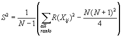
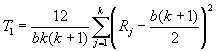
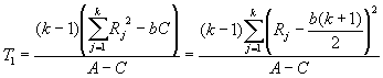
When there are ties, the test statistic T is
S2 is
the variance of the ranks
If there are no ties, S2
= N (N + 1)/12 and the test statistic
simplifies to
When the number of ties is moderate, this simpler equation
may be used with little difference in the result when compared to the more complex
equation need for ties.
The tables required for the exact distribution of T would be quite extensive considering
that every combination of sample
sizes for a given k would be needed,
multiplied by however many samples k
would be included. Fortunately, if ni are reasonably large, say ni ³ 5, then under the null hypothesis T is distributed approximately as chi-square with k - 1 degrees of freedom, Ck-1. For k
=3, sample sizes less than or
equal to 5, and no ties, consult tables in Conover (1999).
Reject the null hypothesis Ho
at level a if T is greater than its 1 - a
quantile. This 1 - a
quantile can be approximated by the chi-square Table C-2 with k-1 degrees of
freedom. Otherwise, accept Ho if T is less than or equal to the 1 - a quantile indicating the means of all the samples are
equal in value. The p-value is approximated by the
probability of the chi-square random
variable with k - 1 degrees of freedom exceeding the
observed value of T.
Computational
Example: (Adapted from Montgomery
(1997, p. 144-145)) A product engineer needs to investigate the tensile
strength of a new synthetic fiber that will be used to make cloth for an
application. The engineer is
experienced in this type of work and knows that strength is affected by the
percent of cotton (by weight) used on the blend of materials for the new
fiber. He suspects that increasing the
cotton content will increase the strength, at least initially. For his application, past experience tells
him that to have the desired characteristics the fiber must have a minimum of
about 10% cotton but not more than about 40% cotton.
To conduct this experiment, the engineer decides to use a
completely randomized design, often called a single-factor experiment. The engineer decides on five levels of
cotton weight percent (k samples) and to test five specimens
(called replicates) at each level of cotton content (ni for each sample
is 5) the fibers are made and tested in random order to prevent effects of
unknown “nuisance” variables, e.g., if the testing machine calibration
deteriorates slightly with each test.
The test results of all 25 observations are combined,
ordered, and ranked. Tied values are
given the average of the ranks
that they would have been assigned to them had there been no ties. The test results and the ranks are shown in
the following table.
Table 9: Kruskal-Wallis One-Way Analsis of Variance
by Ranks Test for Cotton Example
|
Weight Percent
of Cotton
|
|
15
|
20
|
25
|
30
|
35
|
|
X1j
|
R (X1j)
|
X2j
|
R (X2j)
|
X3j
|
R (X3j)
|
X4j
|
R (X4j)
|
X5j
|
R (X5j)
|
|
7
|
2.0
|
12
|
9.5
|
14
|
11
|
19
|
20.5
|
7
|
2.0
|
|
7
|
2.0
|
17
|
14
|
18
|
16.5
|
25
|
25
|
10
|
5
|
|
15
|
12.5
|
12
|
9.5
|
18
|
16.5
|
22
|
23
|
11
|
7.0
|
|
11
|
7.0
|
18
|
16.5
|
19
|
20.5
|
19
|
20.5
|
15
|
12.5
|
|
9
|
4
|
18
|
16.5
|
19
|
20.5
|
23
|
24
|
11
|
7.0
|
|
Ri
=
|
27.5
|
|
66.0
|
|
85.0
|
|
113.0
|
|
33.5
|
|
ni
=
|
5
|
|
5
|
|
5
|
|
5
|
|
5
|
|
|
|
|
|
|
|
|
|
|
N = 25
|
An example of how ties are ranked can be seen from the
lowest value, which is 7. Note that
there are three observations that have a value of 7 so these would normally
have ranks 1, 2, and 3. Since they are
tied, they are averaged and each value of 7 gets the rank of 2.0.
The hypothesis
to be tested is
Ho: E
(X1) = E (X2)
= . . . = E (Xk) all of the 5 blended fibers, with different percent
weights of cotton, have mean
tensile strengths that are equal
Ha:
At least one of the 5 blended fiber mean tensile strengths is not equal
to at least one of the other blended fiber mean tensile strengths
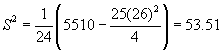
Since there are ties, the variance of the ranks S2
is calculated by
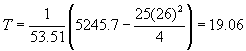
The test statistic
is calculated by
For a critical region of 0.05, the 1 - a
quantile (0.95) of the chi-square distribution
with 5 - 1 = 4 degrees of freedom
from Table C-2 is 9.49. Since T
= 19.06 lies in this critical region, i.e., in the region greater than 9.488,
the null hypothesis Ho is rejected and it is
concluded that at least one pair of the blended fiber tensile strength means is
not equal to each other.
When the Kruskal-Wallis test rejects the null hypothesis,
it indicates that one or more pairs of samples do not have the same means but
it does not tell us which pairs.
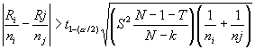
Various sources support different methods for finding the specific pairs
that are not equal, called pairwise comparisons. Conover (1990) discusses using the usual parametric procedure,
called “Fisher’s least significant difference,” computed on the ranks instead
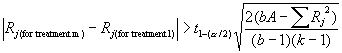
of the data. If, and only if, the null hypothesis is rejected, the
procedure dictates that the population means i and j seem to be
different if this inequality is satisfied.
Ri and Rj
are the rank sums of the two samples being compared. The 1 - a/2
quantile of the t distribution, t1-(a/1),
with N - k degrees of freedom
is obtained from the t distribution
Table C-4. S2 and T are as already defined for the Kruskal-Wallis
test.
For the fiber tensile strength computational example, the
pairwise comparisons between the 15% and the 20% cotton content fibers can be
made by the following computation. For
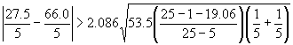
a critical region of 0.05, from Table C-4, the 1 - a/2 quantile (0.975) for the t distribution with
25 -5 = 20 degrees of freedom is
2.086.
Since the inequality is true, it is concluded that the
tensile strength means of the 15% and the 20% cotton content fibers are
different. Notice that since all the
samples are the same size, the right side of this equality will remain constant
for all comparisons. The following
table lists all the pairwise comparisons.
Table 10: Pairwise Comparisons for Cotton Content Example
|
Cotton
Contents
(% by wt)
|
 
|
|
|
15% and 20%
|
7.7
|
4.80
|
|
15% and 25%
|
11.5
|
4.80
|
|
15% and 30%
|
17.2
|
4.80
|
|
15% and 35%
|
1.2
|
4.80
|
|
20% and 25%
|
3.8
|
4.80
|
|
20% and 30%
|
9.4
|
4.80
|
|
20% and 35%
|
6.5
|
4.80
|
|
25% and 30%
|
5.6
|
4.80
|
|
25% and 35%
|
10.3
|
4.80
|
|
30% and 35%
|
15.9
|
4.80
|
All of the pairwise inequalities are true except for two,
the 15% and 35% pair and the 20% and 25%.
Based on the engineers originally stated experience, he suspects that
the 35% fiber may be losing strength which would account for the 15% and 35%
pair having the same tensile strength.
The equal strengths of the 20% and 25% strengths appears to indicate
that little benefit is gained in tensile strength by this raise the cotton
content as compared to, say, the increase from 15% to 20% or from 25% to
30%. Of course, more testing is
probably prudent now that this preliminary information is known.
While this test is said to be for
two dependent samples, it is actually a matched pair that is a single
observation of a bivariate random variable.
It can be employed in “before” and “after” observations on each of
several subjects, to see if the second random variable
in the pair has the same mean as the first one. To be employed more generally, the Wilcoxon Matched-Pairs
Signed-Ranks test requires that each of n
subjects (or n pairs of matched
subjects) has two scores, each having been obtained under one of the two
experimental conditions. A difference
score Di is computed for
each subject by subtracting a subject’s score in condition 2 from his score in
condition 1. Thus, this method reduces the matched pair to a single
observation. The hypothesis
evaluated is whether or not the median of the difference scores equals
zero. If a significant difference
occurs, it is likely the conditions represent different populations.
The Wilcoxon
Matched-Pairs Signed Ranks Test was introduced earlier as a median
(mean) test under the name Wilcoxon Signed-Ranks Test for a Single Independent
Sample. In that test, pairs were formed
between a value in the sample and the sample
median (mean). Here, the test is
extended to an experiment design
involving two dependent samples. Other
than the forming of the pairs, the rest of the procedures remain the same.
ASSUMPTIONS OF WILCOXON
MATCHED-PAIRS SIGNED-RANKS TEST FOR TWO DEPENDENT SAMPLES
1. The
sample of n subjects is a random sample
from the population it
represents. Thus, the Dis are mutually independent.
2. The
Dis all have the same
mean.
3. The
distribution of the Dis is symmetric.
4. The
measurement scale of the Dis
is at least interval.
The data
consist of n observations (x1, y1), (x2, y2), . . . , (xn, yn) on the respective bivariate random variables (X1, Y1), (X2, Y2), . . . , (Xn, Yn).
A. Two-sided test
Ho: E
(D) = 0 or E
(Yi) = E (Xi)
Ha:
E (D) ¹ 0
B. Upper-sided test
Ho: E
(D) £
0 or E (Yi) £ E (Xi)
Ha:
E (D) > 0
C. Lower-sided test
Ho: E
(D) ³
0 or E (Yi) ³ E (Xi)
Ha:
E (D) < 0
The ranking is done on the absolute values of the
differences between X and Y
All differences of zero are omitted. Let the number of pairs remaining be denoted
by n’, n’ < n. Ranks from 1 to n’ are assigned to the n’
differences. The smallest absolute
difference |Di | is ranked
1, the second smallest |Di |
is ranked 2, and so forth. The largest
absolute difference is ranked n’. If groups of absolute differences are equal
to each other, assign a rank to each equal to the average of the ranks they would have otherwise been
assigned.
Although the absolute difference is used to obtain the
rankings, the sign of Di
is still used in the test
statistic. Ri, called the signed rank, is defined as follows:
Ri = the rank assigned to |Di | if Di is positive.
Ri = the negative of the rank assigned to |Di | if Di is negative.
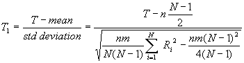
The test statistic
T+ is the sum of the
positive signed ranks when there are no ties and n’ < 50. Lower quantiles
of the exact distribution of T+ are given in Table C-8,
under the null hypothesis that
the Di s have mean 0.
Based on the relationship that the sum of the absolute
differences is equal to n’ (n’ + 1) divided by 2, the upper
quantiles wp are found by the relationship
If there are many ties, or if n’ > 50, the normal approximation test statistic T is used which uses all of the signed ranks, with their + and -
signs. Quantiles of the approximate distribution of T are given in a Normal Distribution Table.
For the two-sided test, reject the null hypothesis Ho at level a
if T+ (or T) is less than its a/2
quantile or greater than its 1 - a/2
quantile from Table C-8 for T+
(or the Normal Table C-1 for T). Otherwise, accept Ho indicating the means of the two conditions are
equal.
For the upper-tailed test, reject the null hypothesis Ho at level a
if T+ (or T) is greater than its a
quantile from Table C-8 for T+
(or the Normal Table C-1 for T). Otherwise, accept Ho indicating the mean of Yi
is less than or equal to the mean
of Xi.
For the lower-tailed test, reject the null hypothesis Ho at level a
if T+ (or T) is less than its a
quantile from Table C-8 for T+
(or the Normal Table C-1 for T).
Otherwise, accept Ho
indicating the mean of Yi is greater than or equal
to the mean of Xi.
Computational
Example: (Adapted from Conover
(1999, p. 355)) Researchers wanted to compare identical twins to see if the
first-born twin exhibits more aggressiveness than the second born twin
does. The Wilcoxon Matched-Pairs
Signed-Ranks test is often used where two observations (two variables) are the
matched-pairs for a single subject.
Here it is used where two subjects are the matched pairs for a single
observation (variable). So each pair of
identical twins is the matched-pair and the measurement for aggressiveness is
the single observation.
Twelve sets of identical twins were given psychological
tests that were reduced to a single measure of aggressiveness. Higher scores in
the following table indicate high levels of aggressiveness. The sixth twin set has identical scores so
they are removed from the ranking.
Table 11: Identical Twin Pyschological Test Example
|
Twin Set
|
1
|
2
|
3
|
4
|
5
|
6
|
7
|
8
|
9
|
10
|
11
|
12
|
|
Firstborn Xi
|
86
|
71
|
77
|
68
|
91
|
72
|
77
|
91
|
70
|
71
|
88
|
87
|
|
Second born Yi
|
88
|
77
|
76
|
64
|
96
|
72
|
65
|
90
|
65
|
80
|
81
|
72
|
|
Difference Di
|
+2
|
+6
|
-1
|
-4
|
+5
|
0
|
-12
|
-1
|
-5
|
+9
|
-7
|
-15
|
|
Ranks of |Di|
|
3
|
7
|
1.5
|
4
|
5.5
|
na
|
10
|
1.5
|
5.5
|
9
|
8
|
11
|
|
Ri
|
3
|
7
|
-1.5
|
-4
|
5.5
|
na
|
-10
|
-1.5
|
-5.5
|
9
|
-8
|
-11
|
The hypotheses to be tested are the lower-sided test
Ho: E
(D) ³
0 or E (Yi) ³ E (Xi) or E (Xi)
£ E (Yi): The firstborn twin (E (Xi)) does
not tend to be more aggressive than the second born twin (E (Yi))
Ha:
E (D) < 0 or
E (Yi)
< E (Xi) or E (Xi) > E (Yi):
The firstborn twin tends to be more aggressive than the second born
twin.
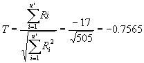
There are several ties so the test statistic is
For a critical region of size 0.05, the a
quantile from the standard normal Table C-1
is -1.6449. Since T = -0.7565 is not in this critical
region, the null hypothesis Ho is accepted and it is
concluded that the firstborn twin does not exhibit more aggressiveness than
does the second born twin.
Traffic Example: In a
comparative study of modeling approaches for traffic flow forecasting (Smith
and Demetsky, Journal of Transportation
Engineering, V.123, N.4, July/August, 1997), researchers needed to assess the
relative merits of four models they developed.
These traffic-forecasting models were developed and tested using data collected at two sites in
Northern Virginia. Two independent sets
of data were collected for model
development and model evaluation. The models were estimated using four
different techniques from the development
data: historic average, time-series, neural network, and nonparametric regression (nearest
neighbor).
One of the comparative measures used was the absolute error of the models. This is simply how far the predicted volume
deviates from the actual observed volume, using the model evaluation data.
The data were paired by
using the absolute error
experienced by two models at a given prediction time. The Wilcoxon Matched-Pairs Signed-Ranks Test for dependent
samples was used to assess the statistical difference in the absolute error between any two models. This test was chosen over the more
traditional analysis of variance
approach (ANOVA) because the distribution of the absolute errors is not normal,
an assumption required for ANOVA.
One of the models could not be tested because of insufficient data,
leaving three models to be compared.
These models were compared using three tests, representing all combinations
of comparison among three models. Two
hypotheses were tested for each pair of models:
Ho: m1 -m1 = 0
Ha: | m1 -m1 ¹ 0 | (note: the paper states the
alternate hypothesis as m1 -m1 > 0, which is incorrect
for a two-sided test, but its evaluation is correct meaning that it actually evaluated as if it were a two-sided
test.)
A 1% or less level of significance
was used as being statistically significant.
Data from two sites were used, so the three tests were performed
twice. Although not stated specifically
in the paper, it appears that the sample
size was greater than 50. This
allowed the researchers to use the normal approximation test statistic. For each of the two sites, the nonparametric
regression (nearest neighbor)
model was the preferred model. Using
this evidence, as well as other qualitative and logical evidence, the
researchers were able to draw the conclusion that nonparametric regression (nearest neighbor)
holds considerable promise for application to traffic flow forecasting.
A technique employed in this evaluation has universal application. The test selected only compares two
samples. Therefore if more samples need
to be compared, one can perform a series of tests using all the possible
combinations for the number of samples to be evaluated. It should be noted that often more
sophisticated methods for testing multiple samples simultaneously usually
exist. Often these tests require more detailed
planning prior to collecting the data.
Unfortunately many researchers collect data with only a vague notion of
how the data will ultimately be
analyzed. This often limits the statistical methods available to
them--usually to their detriment. The
next test in this manual, Friedman Two-Way Analysis of Variance by Ranks Test for several
dependent variables, is an alternative that may have provided more
sophisticated evaluation for these researchers, if their data had been drawn
properly.
The situation arises where a matched-pair is too limiting
because more than two treatments (or variables) need to be tested for
differences. Such situations occur in
experiments that are designed as randomized
complete block designs. Recall that
the Kruskal-Wallis One-Way Analysis of Variance by Ranks test was applied to a completely randomized design; this
design, which relies solely on randomization, was used to cancel distortions of
the results that might come from nuisance
factors. A nuisance factor is a variable that probably has an
effect on the response variable, but is not of interest to the analyst. It can be unknown and therefore
uncontrolled, or it can be known and not controlled. However, when the nuisance factor is known and controllable, then
a design technique called blocking
can be used to systematically eliminate its effects. Blocking means that all the treatments are carried out on a
single experimental unit. If only two
treatments were applied, then the experimental unit would contain the
matched-pair treatments, which was the subject of the previous section on the
Wilcoxon Matched-Pairs Signed-Ranks test.
This section discussed a test used when more than two treatments are
applied (or more than two variables are measured).
The situation of several related samples arises in an experiment that is designed to
detect differences in several possible treatments. The observations are arranged in blocks, which are groups of
experimental units similar to each other in some important respects. All the treatments are administered once
within each block. In a typical
manufacturing experiment, for example, each block might be a piece of material bi that needs to be treated
with several competing methods xi. Several identical pieces of material are
manufactured, each being a separate block.
This would cause a problem if a completely randomized design were used
because, if the pieces of material vary, it will contribute to the overall variability of the testing. This can be overcome by testing each block
with each of the treatment. By doing
this, the blocks of pieces of material form a more homogeneous experimental unit
on which to compare the treatments.
This design strategy effectively improves accuracy of the comparisons among treatments by eliminating
the variability of the blocks
or pieces of materials. This design is
called a randomized complete block design.
The word “complete” indicates that each block contains all of the
treatments.
The randomized complete block design is one of the most
widely used experimental designs. Units
of test equipment or machinery are often different in their operating
characteristics and would be a typical blocking factor. Batches of raw materials, people, and time
are common nuisance sources of variability
in transportation experiments that can be systematically controlled through
blocking. For example, suppose you want
to test the effectiveness of 4
sizes of lettering on signage. You
decide you will measure 10 people’s reactions and want a total sample size of 40. This allows 10 replicates of each size of
lettering. If you simply assign the 40
tests (10 for size 1, 10 for size 2, 10 for size 3, and 10 for size 4) on a
completely random basis to the 10 people, the variability of the people will
contribute to the variability
observed in the people’s reactions.
Therefore, each person can be blocked by testing all four lettering
sizes on each person. This will allow
us to compare the lettering sizes without the high variability of the people confusing the results of the
experiment.
The parametric test method for
this situation (randomized complete block design) is called the single-factor within-subjects analysis of
variance or the two-way analysis of
variance. The nonparametric
equivalent tests depend on the ranks of the observations. An extension of the Wilcoxon Matched-Pairs
Signed-Ranks test for two dependent samples to a situation involving several
samples is called the Quade Test. Dana
Quade first developed it in 1972. The
Quade test uses the ranks of the observations within each block and the ranks
of the block-to-block sample ranges to develop a test statistic.
An alternate test
to the Quade test was developed much earlier (1937) by noted economist Milton
Friedman. The Friedman test is an
extension of the sign test and is better known. Which test to use depends on the number of treatments. Conover (1999) recommends the use of the
Quade test for three treatments, the Friedman test for six or more treatments,
and either test for four or five treatments.
These recommendations are based on the power
of the tests for various levels of treatments.
Since the Friedman test is useful for a much larger range
of treatments, it is discussed in this section. Discussion of the Quade test is presented in Conover (1999, p.
373-380).
ASSUMPTIONS OF FRIEDMAN TWO-WAY
ANALYSIS OF VARIANCE BY RANKS TEST FOR SEVERAL DEPENDENT VARIABLES
1. The
multivariate random variables are mutually independent. In other words, the results within one block
do not affect the results within any of the other blocks.
2. Within
each block the observations may be ranked according to some criterion of
interest.
The data consist of b
mutually independent observations where each observation contains k random variables (Xi1, Xi2,
. . . ,Xbk). The observations are designated as b blocks, i = 1, 2, . . . , b. The random variable Xij
is in block i and is subjected
to treatment j (or comes from population j). The data can be arranged in a matrix
with i rows for the blocks and j columns for the treatments
(populations).
Table 12: Friedman Two-Way Analysis of Variance Table for Ranks Test
for Several Dependent Variables
|
|
treatment 1
|
treatment 2
|
. . .
|
treatment k
|
|
block
1
|
X1,1
|
X1,2
|
.
. .
|
X1, k
|
|
block
2
|
X2,1
|
X2,2
|
.
. .
|
X2, k
|
|
. . .
|
.
. .
|
.
. .
|
.
. .
|
.
. .
|
|
block
b
|
Xb,1
|
Xb,2
|
.
. .
|
Xb, k
|
Ho: E
(X1j) = E (X2j) = , . . . , = E
(Xbj); All of the b
treatment (population) means are equal, i.e., each ranking of the random
variables within a block is equally likely.
Ha:
At least one of the b
treatment (population) means is not equal to at least one of the other
treatment (population) means
Current research
reported by Conover (1999, p. 370) has found the approximation of the Friedman
test statistic by the
chi-square distribution is sometimes poor.
This supports a modification to the Friedman test statistic, which
allows the F distribution to be used as its
approximation with better results.
First rank the treatments (populations) within each block
separately. The smallest value within a
block is assigned rank 1 continuing through the largest value, which is
assigned rank k. Use average ranks in case of ties. Calculate the sum of the ranks Rj, for each treatment (population)
Then calculate Friedman’s statistic
When there are ties, T1
needs to be adjusted by A and C
After adjusting the test statistic T1
for ties, it becomes
Now the final test statistic T2 is calculated by modifying T1 so it can be approximated by the chi-square
distribution
When the null hypothesis
is true, the exact distribution of T2
is difficult to determine so its quantiles are approximated by the F distribution with numerator degrees of freedom dfnum
= k - 1 and denominator degrees of freedom dfden = (b - 1)(k - 1).
Reject the null hypothesis Ho
at level a if T2 is greater than its 1 - a
quantile. This 1 - a
quantile s approximated by the F distribution Table C-5 with dfnum = k - 1 and dfden
= (b - 1)(k - 1). Otherwise, accept Ho if T2 is less than or equal to the 1 - a
quantile indicating the means of all the samples are equal in value. The approximate p-value can also be approximated from the F distribution
table. As one might suspect the
approximation gets better as the number of blocks b gets larger.
Computational
Example: (Adapted from Montgomery
(1997, p. 177-182)) A machine to test hardness can be used with four different
types of tips. The machine operates by
pressing the tip into a metal specimen and the hardness is determined by the
depth of the depression. It is
suspected that the four tip types do not produce identical readings so an experiment is devised to check
this. The researcher decides to obtain
four observations (replicates) of each tip type. A completely randomized single-factor design would consist of randomly
assigning each of the 16 tests (called runs) to an experimental unit (a metal
specimen). This would require 16
different metal specimens. The problem
with this design is that if the 16 metal specimens differed in hardness, their
variability would be added to any variability
observed in the hardness data caused by the tips.
To overcome the potential variability in the metal specimens, blocking can be used to
develop a randomized complete block design experiment. The metal specimens will be the blocks. Each block will be tested with all four
tips. Therefore, only four metal
specimens will be needed to conduct the 16 total tests. Within each block, the four tests need to be
conducted in random order. The observed
response to the tests is the Rockwell C scale hardness minus 40 shown in the
following table.
Table 13: Randomized Complete Block Design for Metal
Specimens Example
|
|
treatment (tip type) 1
|
|
treatment (tip type) 2
|
|
treatment (tip type) 3
|
|
treatment (tip type) 4
|
|
|
|
value
|
rank
|
value
|
rank
|
value
|
rank
|
value
|
rank
|
|
block specimen 1
|
9.3
|
2
|
9.4
|
3
|
9.2
|
1
|
9.7
|
4
|
|
block specimen) 2
|
9.4
|
2.5
|
9.3
|
1
|
9.4
|
2.5
|
9.6
|
4
|
|
block specimen 3
|
9.6
|
2
|
9.8
|
3
|
9.5
|
1
|
10.0
|
4
|
|
block specimen4
|
10.0
|
3
|
9.9
|
2
|
9.7
|
1
|
10.2
|
4
|
|
Rj (totals)
|
|
9.5
|
|
9
|
|
5.5
|
|
16
|
Since there are ties, first compute A and C
Next compute the Friedman test statistic T1
using the formula adjusted for ties
Finally modify T1
to obtain the test statistic T2
For a critical region of 0.05, the 1 - a
quantile (0.95) of the F distribution with dfnum = k - 1 = 3 and dfden
= (b - 1)(k - 1) = (3)(3) = 9 from Table C-5 is 3.86. Since T2
= 8.4148 lies in this critical region, i.e., in the region greater than 3.86,
the null hypothesis Ho is rejected and it is
concluded that at least one tip type results in hardness values that are not
equal to at least one other tip type.
From Table C-5, the p-value is
less than 0.01. This means the null
hypothesis Ho could have
been rejected at a significance
level as small as a =
0.01 (and even smaller, but most tables don’t have values any smaller).
When the Friedman test rejects the null hypothesis, it
indicates that one or more treatments (populations) do not have the same means
but it does not tell us which treatments.
One method to compare individual treatments is presented by Conover
(1999, p. 371). This method concludes
that treatments l and m are different if the following
inequality is satisfied.
Ri and Rj
are the rank sums of the two treatments (samples) being compared. The 1 - a/2 quantile of the t
distribution, t1-(a/1),
with (b - 1)(k - 1) degrees of
freedom is obtained from the t distribution,
Table C-4. A is as already defined
for the Friedman test.
If there are no ties, A
in the above inequality simplifies to
Multiple comparisons for the hardness testing machine
computational example can be made by first computing the right side of the
inequality. For a critical region of 0.05, from Table C-4, the 1 - a/2
quantile (0.975) for the t distribution with (4 - 1)(4 - 1) = 9 degrees of freedom is 2.262.

It can be concluded that any two-tip types whose rank sums
are more than 4.8280 are unequal.
Therefore, tip types which yield mean hardness values different from
each other are types 1 and 4, types 2 and 4, and types 3 and 4. No other differences are significant. This means that types 1, 2, and 3 yield
identical results (at a
= 0.05) while type 4 yields a significantly higher reading than any of the
other three tip types.
Sometimes it is inconvenient or impractical to administer
all the treatments to each block.
Perhaps there is limited funds or perhaps the number of treatments is
simply too large to administer to each block.
When blocking is used, but each block does not receive every treatment,
it is called a randomized incomplete
block design. Furthermore, when certain
simple treatment scheme conditions are met to aid analysis, the design is
called a balanced incomplete block
design. The parametric analysis
methods for this type of design are discussed in detail in Montgomery (1997, p.
208-219). When the normality
assumptions are not met, a test developed by Durbin in 1951 may be used. It is a rank test to test the null hypothesis that there are no
differences among treatments in a balanced incomplete block design. For details about the Durbin test, see
Conover (1999, p. 387-394).
A measure of association
describes the relationship between variables.
Another term often used is correlation, which is essentially synonymous
with association. Measures of association or correlation are
descriptive statistical measures that attempt to quantify the degree of
relationship between two or more variables.
After calculating a measure of association, it is usually possible to
devise an inferential test to evaluate a hypothesis about the measure of association. This section deals with nonparametric
measures of association and
tests for independence, i.e., measures and tests that do not rely on knowing
the parameters of the underlying distributions of the variables being
studied. The focus is on comparing two
variables, called a bivariate measure of association.
Examples:
An analyst or engineer might be interested in assessing the evidence regarding
the relationship (independent or not) between two variables, e.g., two
variables such as:
1. Airport site evaluation ordinal
rankings of two sets of judges, i.e., citizens and airport professionals.
2. Neighborhood districts residents’
use of a regional mall for purposes of planning transit routes.
3. Accidents before and during roadway
construction to investigate whether factors such as roadway grade, day of week,
weather, etc. have an impact on crashes.4.
Area type and speed limit--as well as other variable pairs--to eliminate intercorrelated dependent
variables for estimating models that predict the number of utility pole accidents.
As the reader will recall, there are four types of
measurement scales that can be used to quantify data. These are called nominal, ordinal, interval, and ratio scales,
listed from “weakest” to “strongest.”
Thus the ratio scale is
the strongest and gives us the most quantitative information of any of the
scales while nominal gives us the least information. This hierarchy allows for data to be transformed to a lower level, but they can’t be
transformed to a higher one. These
measurement scales are defined in detail in Appendix A.
Measures of Association:
The most commonly used measure of correlation is Pearson’s
product-moment correlation
coefficient, usually denoted by r.
Pearson’s r was developed in 1896 and
1900 by Karl Pearson (1857-1936), an English mathematician. Pearson was a pioneer of statistics who also developed the
chi-square test that is used extensively in nonparametric methods. Pearson’s r, however, is a random
variable and therefore has a distribution
function. This distribution function depends on
the bivariate distribution
function of the two variables being tested.
Specifically, it assumes that each of the two variables and their linear
combination are normally distributed--called a bivariate normal distribution. Therefore, Pearson’s r is not useful as a test statistic in nonparametric methods. Fortunately, other measures are available
which do not assume a bivariate normal distribution of the two variables, which are detailed in
this section.
In order for a quantitative measure of association to be useful, it must
be scaled in a manner that implicitly yields information by its value. Traditionally (but there are exceptions),
the value calculated will fall between 0 and +1 or between -1 and +1. A 0 value indicates no relationship between
the two variables being compared. A
value of -1 or +1 indicates a maximum relationship between the two
variables. The closer to an absolute
value of 1 (either +1 or -1), the stronger the measure of association. When the measure can have a value from -1 to
+1, the negative values indicate an inverse relationship (one increases as the
other decreases) while the positive values indicate a positive relationship
(both increase or decrease together).
It is important to remember that these relationships are
only associations and do not imply causation.
One cannot say, based on a strong measure of association/correlation,
that one variable causes
another variable. It is possible such a
causal relationship exists but it cannot be discerned by using a measure of
association/correlation. Such a result
could have been caused by an extraneous (often called a confounding) variable or variables that were
not measured by the researcher. These
extraneous variables could be responsible for the observed correlation between the two
variables.
Tests for Independence:
Measures of association/correlation are not inferential tests. But as stated earlier, after calculating a
measure of association, it is usually possible to devise an inferential test to
evaluate a hypothesis about the
measure of association. As the reader
will recall, hypothesis testing
is the process of inferring from a sample whether or not a given statement
about the population appears to be true.
The hypotheses discussed in this section can generally be employed in
tests for independence. This allows us
to determine whether an association
between two variables is due to chance or is highly unlikely to have occurred
by chance. Whereas a measure of association gives a quantitative
measure of the relationship between two variables, its interpretation is
subjective. The interpretation of a
test for independence allows the researcher to estimate a probability that the
observed data occurs when the
null hypothesis is true (the null hypothesis
is usually that the variables are independent). For example, there is less than a 5% probability that a specific data sample of two variables would occur given that the two data
variables are independent. In this
example, since there is less than a 5% probability of the specific data occurring by chance alone, the
given condition of independence could be rejected (at the 5% significance level). This means that the alternative hypothesis would be accepted,
i.e., the two variables are not independent and, thus, a relationship between
them exists.
The Test for Independence using nominal data discussed in the next section
uses a r x c contingency table to
explore whether two variables within a sample are independent or not. But sometimes instead of testing a hypothesis regarding independence, the analyst simply want
to express the degree of dependence shown in a particular contingency table. The most widely used measure of dependence
(also called a Measure of Association) for an r x c contingency table is Cramer’s
Contingency Coefficient. Sometimes
called Cramer’s phi coefficient or simply Cramer’s coefficient, this measure of
dependence was first suggested by Harold Cramer (1893-1985), a Swedish
mathematician and chemist, in 1946.
The coefficient is based on the test statistic T developed in the
Chi-square Test for Independence. This
test is detailed in the following section and all of its underlying assumptions
apply to Cramer’s Contingency Coefficient.
A random sample
of size N is obtained by the
researcher. The observations may be
classified according to two variables.
The first variable has r categories (rows) and the second variable has c categories (columns). Let
Oij be the number of observations
associated with row i and column j simultaneously (a cell). The cell counts Oij are arranged in the following form, which is called a r x c
contingency table.
The total number of observations from all samples is
denoted by N. The number of observations in the jth column is denoted by Cj,
which is the number of observations that are in row j (meaning category j of
the second variable). The number of observations in the ith row is denoted by Rj, which is
the number of observations that are in row i
(meaning category i of the first
variable).
Table 14: Contingency
Table for Two Variables
|
|
Column 1
|
Column 2
|
. . .
|
Column j
|
. . .
|
Column c
|
Row
Totals
|
|
Row 1
|
O1 1
|
O1 2
|
. . .
|
O1 j
|
. . .
|
O1 c
|
R1
|
|
Row 2
|
O2 1
|
O2 2
|
. . .
|
O2 j
|
. . .
|
O2 c
|
R2
|
|
. . .
|
|
|
|
|
|
|
. . .
|
|
Row i
|
O i 1
|
O i 2
|
. . .
|
O i j
|
. . .
|
O i c
|
Ri
|
|
. . .
|
|
|
|
|
|
|
. . .
|
|
Row r
|
O r 1
|
O r 2
|
. . .
|
O r j
|
. . .
|
O r c
|
Rr
|
|
Column Totals
|
C1
|
C2
|
. . .
|
Cj
|
. . .
|
Cc
|
N
|
The difficulty with directly using the test statistic T for the Chi-square Test for Independence is its lack of a common
scale. The test statistic T is an estimate of a chi-square value. Chi-square values cannot be directly compared because their
probabilities vary depending upon their degrees of freedom, which varies from sample to sample. Cramer’s approach lessens this dependency on
the degrees of freedom by
dividing T by the maximum value that T can have. The methodology for developing the test statistic T for the Chi-square Test for Independence is detailed in the
following section and not repeated here.
However, it is easily seen by examining the test statistic T formula
that large values of T arise as the
difference in cell counts (Oij
- Eij) becomes more
pronounced. By examining extremely uneven contingency tables, a general
rule was developed for the maximum value of T
being N(k - 1), where k is the
smaller of the number of categories for the two variables being considered and N is the total number of
observations. Therefore, when T is divided by the approximation of the
maximum value of T, the result is a
useful coefficient C having a common
scale. Current convention uses the
square root form.
If the result is close to 1.0, the contingency table indicates a
strong dependency between the two variables; when it is close to 0.0, the
numbers across each row (first variable) are in the same proportions to each
other as the column totals (second variable) are to each other--indicating independence.
It should be noted that while measures of association have a quantitative
scale, their interpretation is subjective.
The interpretation can be improved by performing the Test for Independence
on the contingency table as
detailed in the following section. This
test determines if the test statistic
T (estimate of chi-square value) is
statistically significant at a given level of significance. The Measure of Association computed for the contingency table, in this
case Cramer’s Contingency
Coefficient will be significant at this same level of significance. Finally, it is important to note once more
that these relationships are only associations and do not imply causation.
Whereas Cramer’s Contingency Coefficient is the most widely used measure of
dependency for r x c contingency tables, other measures
are sometimes used. One widely know measure
is Pearson’s Coefficient of Mean
Square Contingency sometimes simply called Pearson’s Contingency
Coefficient. Detailed information on
this measure and others is available from Conover (1999, p231-233) or Sheskin
(1997, p.243-244). The choice of a
measure of dependency is a personal choice.
1) The
sample of N observations is a
random sample.
2) Each
observation may be categorized into exactly one of the r categories for one variable
and c categories for the other variable (i.e., the r categories are mutually exclusive and collectively exhaustive as are the c categories)
3) The
number of observations that fall into each r
category for one variable or
for each c category for the other variable are not predetermined by
the researcher prior to the data
collection phase of a study.
4) Each
cell contains at least 5 observations (see the discussion under “Trouble
shooting” about possible remedies if this assumption is violated).
Safety Example: In a
reexamination of a study to determine whether to use red left turn arrows
instead of red balls (Kullback and Keegel, Journal of Transportation Engineering, V.111,
N.4, July, 1985), researchers challenged the conclusions of the previous study
because of inappropriate use of the Chi-square Test for Independence. The original study had used a contingency table with 72
cells. However 30 of these cells had
zero observations, making the use of this test highly problematic.
5) The
measurement scale is at least nominal.
The data
consist of an r x c contingency table, as prepared for Cramer’s Contingency Coefficient detailed in
the previous section.
Let the probability of a randomly selected value from the ith population being classified in the
jth class be denoted by pi j, for i = 1, 2, . . . , r, and j = 1, 2, . . . , c.
Ho: The
two variables are independent of each other, i.e., the rows and columns
represent two independent classification schemes. (Oi j = Ei
j, for all cells).
Ha:
The two variables are not independent of each other. (Oi j ¹
Ei j, for all cells).
The null hypothesis
can be stated as the event “an observation is in row i” is independent of the event “that same observation is in column j,” for all i and j. By definition, when two events are
independent, the probability of both occurring is simply the product of their
probabilities. Thus, for any cell,
assuming the null hypothesis is
true (the variables are independent), the expected
number of observations is the product of their category probabilities. The row probability is simply the row total
divided by all the observations, P (row
i) = Ri /N. Similarly,
the column probability is the column total divided by all the observations, P (column j) = Cj /N. Therefore the expected number of
observations in a cell is the cell probability times the total number of
observations in all the cells
Where Ei j
represents the expected number of observations in cell (i, j) when Ho is true. The test statistic T is
given by
The approximate distribution of T
is the chi-square distribution
with (r - )(c - 1) degrees of freedom. Therefore the critical region of
approximate size a significance level corresponds to
values of T greater than x1- a,
the (1 - a)
quantile of a chi-square random
variable with (r - 1)(c - 1) degrees of freedom, obtained from
the Chi-square distribution, Table C-2. One rejects Ho if T exceeds
x1-a
(meaning that an observation’s categorization on the first variable is associated (i.e., not
independent) with the categorization on the second variable). Other wise the analyst accepts Ho (meaning the two variables
are independent).
Transit Example: In the design
of off-peak transit routes (Ross and Wilson, Transportation Engineering
Journal, V.103, N.TE5, September 1977), researchers in Cedar Rapids, Iowa,
developed a routing technique to identify the trade area of major trip attractors
and design the transit routing to serve areas of high potential within the
trade area. To demonstrate the effectiveness of the technique, the
researchers collected data for a
non-CBD (central business district) regional mall and its trade area. The data captured demographic characteristics of the mall’s
patrons and characteristics of their trips to the mall during off-peak
hours. Screening methods were used to
eliminate from evaluation traffic zones of very low potential transit ridership
to the mall, essentially all areas outside a 10-minute travel time to the
mall. Additionally, low population traffic zones within
the 10-minute limit were also dropped, typically rural zones. The remaining traffic zones were aggregated
into four districts conducive to efficient transit routing to the mall.
Several questions were posed in the form of two hypotheses and tested
using the Chi-square Test for Independence for nominal data:
Ho: The two variables are independent of each other.
Ha: The two variables are not independent of each
other.
A 1% or less level of
significance was used as being statistically significant and the p-values
were reported when the level of significance
was greater than 1%.
One example of a question explored was the preference of district
residents for shopping at the mall when compared to the CBD. The responses to this choice question were
that they shopped (1) more, (2) the same, or (3) less in the CBD than in the
mall. Since there were four districts
being evaluated, the researchers set up a 3 by 4 contingency table. The null hypothesis is that the rows (level of shopping at the mall)
are independent of the columns (the district in which the shopper lived). This was rejected at a degree of significance of 0.01. This is interpreted as follows. Given that
the data are independent, there
is less than a 1% chance that the large differences between the expected and
observed values occurred by chance alone.
Therefore the alternate hypothesis
is accepted: the level of shopping is different among the districts. Several other questions were explored in a
similar manner: (1) are the trip frequencies the same by district (no), (2) are
the planned versus unplanned trips to the mall the same by districts (yes with
a p-value = 0.58), (3) are the previous locations of the mall patrons just
before coming to the mall the same by district (yes with a p-value of 0.70),
(4) are the trip making rates per occupied dwelling unit the same by district
(yes with a p-value > 0.70), and then (5) for each zone within a district,
are the trip making rates per occupied dwelling unit the same (results varied
by zone).
From these tests, the researchers were able to draw these general
conclusions:
1. After dropping the lowest use district, all
three remaining districts appear to be producing trips to the mall as a
function of the number of occupied dwelling units in the districts.
2. In two of the districts at least one zone
produces trips at a rate different than would be expected if all trip rates
were equal.
Nonparametric techniques generate p-values without making
any assumptions about the distributions.
However, they do rely on approximate solutions. Recall the noted nonparametric authority
W.J. Conover’s words: “nonparametric methods use approximate solutions to exact
problems, while parametric methods use exact solutions to approximate
problems.” These approximations tend to
become better as the sample size
gets larger because it usually approaches its solution asymptotically or as
some say, the law of large numbers comes into play. So when samples sizes are sufficiently large the approximations
are usually quite good.
For both the Chi-square Test for Independence and the
Chi-square GOF test, the exact distribution
of the test statistic is very
difficult to find and classically is almost never used. The asymptotic chi-square approximation for
the test statistic is satisfactory if the expected values in the test statistic are not too small. However the exact distribution can be found, and has been used for some time
for small contingency tables, e.g., a 2 by 2 contingency table, where the computations
required were manageable. The
computations for larger size contingency
table are difficult computationally.
With the advent of modern computers, however, such computations are
possible and may provide a more useful method when testing small size
samples. These computations are still a
nontrivial task and rely on special algorithms. Cyrus R. Mehta and Nitin R. Patel are two researchers who have
developed such special algorithms and have published their work in this
field. They report that software
support for their methods is available in many standard packages including
StatXact-3, LogXact-2, SPSS Exact Tests, and SAS Version 6.11. More statistical software publishers will
probably add this capability as it becomes more recognized. One should consult these software providers
for more information.
Kendall’s Tau (t)
- Measure of Association for Ordinal, Interval, and Ratio Scale Data
Kendall’s Tau is of a type that can be called measures of
rank correlation. Compared to measures
of association for nominal scale
data, these measures use the additional information contained in ordinal,
interval, and ratio scale data in their computation. In general, this additional information provides tests with
greater power without having to
make the assumptions about the distribution
of the test statistics as is the case for parametric tests (e.g., the widely
used Pearson’s product moment correlation coefficient). Rank correlation methods use the ranks (order) attributed to the
data values rather than the
values themselves resulting in nonparametric tests.
1) P (X = x) < 1 which is a trivial
assumption since it is unlikely the parent population that the sample is drawn from will have only one
member (number). This assumption,
however, allows this test to be valid for all types of populations, whether
continuous, discrete, or mixtures of the two.
2) The
measurement scale is at least ordinal.
The data
consist of a random sample of
size n having two variables (X, Y).
Slightly different versions of Kendall’s Tau are used by
different researchers that require different tables. Described here is the
method used by Conover (1990, p.319-323, TableA11 p.543). Two observations, for example (10.4, 0.6)
and (13.9, 1.1), are called “concordant” if both members (variables) of one
observation are larger than their respective members of the other
observation. Let Nc be the number of concordant pairs of observations out
of the nC2 possible
pairs. A pair of
observations, such as (10.4, 0.6) and (14.2, 0.3), are
called “discordant” if the two numbers in one observation differ in opposite
directions (one negative and one positive) from the respective members in the
other observation. Let Nd be the total number of
discordant pairs of observations. Pairs
with ties between respective members are counted differently, as described
later. Recall nCr =
(n!) / (r! (n - r)!) are all the number of ways in which
r objects can be selected from a set
of n distinct objects. Therefore, the n observations may be paired nC2
= (n!) / (2! (n - 2)!) = n (n - 1) / 2 different
ways. Thus, the number of concordant
pairs Nc plus the number
of discordant pairs Nd
plus the number of pairs with dies will add up to n (n - 1) / 2. The measure of correlation (association) when there are not ties is
If all pairs are concordant, then Kendall’s Tau equals
1.0; when all pairs are discordant, it equals ‑1.0.
Ties: In equation form, a pair of observations
(X1, Y1) and (X2, Y2) is concordant if (Y2 - Y1)
/ (X2 - X1) > 0 and discordant if (Y2 - Y1)
/ (X2 - X1) < 0. If
X1 = X2 the
denominator is zero so no comparison can be made. But when Y1 = Y2 (and X1 ¹ X2), then (Y2 - Y1) / (X2
- X1) = 0. In this case the pair should be counted as
one-half (1/2) concordant and one-half (1/2) discordant. While this makes no difference in the
numerator of Kendall’s Tau because the one-half terms cancel when computing Nc - Nd, it does change the way Tau should be computed. In the case of ties, the measure of association (correlation) is
This version of Kendall’s Tau has the advantage of
achieving +1 or -1 even if ties are present.
This version is sometimes called the “gamma coefficient.”
If the result is close to 1.0, the data indicate a strong positive
association/correlation. This means the
larger values of X tend to be paired
with the larger values of Y and the
smaller values of X tend to be paired
with the smaller values of Y. If the result is close to -1.0, the data indicate a strong negative
association/correlation. This means the
larger values of X tend to be paired
with the smaller values of Y and the
smaller values of X tend to be paired
with the larger values of Y. A result close to 0.0 indicates the values
of X seem to be randomly paired with
the values of Y, and hence indicate
that X and Y are independent. However,
independence has not been statistically tested so the most the analyst can say
is that the variables are uncorrelated.
To statistically test the association (or lack of), the Test of Independence in the next
section needs to be made. Once that is
made, however, and assuming the test is statistically significant at a given
level of significance, then Kendall’s Tau will be significant at this same
level of significance. As with all
Measures of Association, Kendall’s Tau only measures an association between two variables
and do not imply that one causes the other.
Computational
Example: (Adapted from Conover
(1999, p.320)) Suppose the analyst collected twelve observations, each having
two variables for each observation. The
analyst wants to determine the Measure of Association using Kendall’s Tau between two variables. One
of the variables is denoted as X (it
doesn’t matter which one), and the other variable Y. For ease of calculation, the observations
are ordered on their X variable and calculate their
concordant and discordant pairs as shown in the following table. Included are
the ranks of the variables, which some people find easier to use when
comparing. You can use the values
directly or their ranks to make the comparisons. Ranking of ties uses their average rank.
By arranging the data in increasing values of X, each Y may be compared
with only those Ys below it. In this manner each pair is only considered
once and the comparisons can be done by hand fairly quickly. Using the pair (560, 3.2) with ranks (5,
1.5) as an example, the pair relationships are found by comparing 3.2 (or rank
1.5) with the following Ys of 3.2,
3.8, 3.5, 4.0, 3.9, and 4.0 (or with ranks 1.5, 9, 5, 11.5, 10, and 11.5). In 5 comparisons the second Y is larger (concordant), in no cases is
the second Y smaller (discordant),
and in one case there is a tie (1/2 concordant and 1/2 discordant). Note that the two pairs where 560 is tied
with the second X are not counted.
Table 15: Kendall’s Tau Measure of Association between Two Varaiables
|
Values
(Xi,Yi)
|
Ranks
(Ri,Ri)
|
Concordant Pairs
Below
(Xi,Yi) and (Ri,Ri)
|
Discordant Pairs
Below
(Xi,Yi) and (Ri,Ri)
|
|
(530, 3.5(1))
|
( 1, 5)
|
7
|
4
|
|
(540, 3.3)
|
( 2, 3)
|
8
|
2
|
|
(545, 3.7)
|
( 3, 8)
|
4
|
5
|
|
 (560, 3.2(1)) (560, 3.2(1))
|
( 5, 1.5)
|
5.5
|
0.5
|
|
(560, 3.5)
|
( 5, 5)
|
4.5
|
1.5
|
|
(560, 3.6)
|
( 5, 7)
|
4
|
2
|
|
(570, 3.2(1))
|
( 7, 1.5)
|
5
|
0
|
|
(580. 3.8)
|
(8, 9)
|
3
|
1
|
|
 (610, 3.5) (610, 3.5)
|
(9.5, 5)
|
2
|
0
|
|
(610, 4.0(2))
|
(9.5, 11.5)
|
0.5
|
1.5
|
|
(640, 3.9)
|
(11, 10)
|
1
|
0
|
|
(710, 4.0(2))
|
(12,.11.5 )
|
n/a
|
n/a
|
|
|
|
Nc = 44.5
|
Nd = 17.5
|
(1)Yi
tie
(2)Yi tie
Safety Example:
In an evaluation of vehicular crashes with utility poles (Zegeer and
Parker, Transportation Research
Record No. 970, 1984), researchers used data from four states to investigate the effects of various
traffic and roadway variables on the frequency and severity of the
crashes. Several methods were used to
assess these effects including correlation
analysis, analysis of variance
and covariance, and contingency table analysis.
Correlation analysis was conducted to determine if a
relationship existed between the independent and the dependent variables for purposes of determining the best
variables to use in a predictive model.
Similarly correlation
analysis between independent variables was conducted in order to avoid problems
of collinearity in predictive models that occurs when two or more independent
variables in a model are highly
correlated. For variables having
interval and ratio scale data,
the “Pearson correlation
coefficient” was used. For measuring
the association between the
discrete, ordinal independent variables, “Kendall Tau correlation” was
used. For example, a Tau value of 0.727
was reported for the correlation
between area type and speed limit.
There were three area types: urban, urban fringe, and rural. A value of 1.000 would indicate “perfect” correlation between these two variables
while a value of 0.000 would indicates “no” correlation. The researchers made a qualitative
decision that this Tau value was sufficiently close to 1.0 to warrant
eliminating one of the variables--area type--as an independent variable in their predictive
models. After deciding on the “best”
variables to include, the researchers used linear and nonlinear regression analysis to develop
predictive models.
It is important to note that when reporting results,
lack of specificity in naming and/or describing the actual statistical tests
used can cause confusion. In this
example, the researchers reported they used the “Pearson correlation coefficient”, except
for ordinal data, for which they used “Kendall Tau correlation” analysis. In neither case is a statistical reference
given, which would have allowed a reader so inclined to determine the exact statistical
tests that were used. Both Pearson and
Kendall formulated multiple tests for correlation and they are reported in literature and
textbooks under various names. In this
case, “Kendall’s tau” is a relatively unique name but the Pearson correlation coefficient used must
simply be guessed. It is probably
Pearson’s Product Moment Correlation Coefficient, which is arguably the most
widely used correlation
coefficient for interval and ratio scale variables when developing linear regression models. An alternate method for providing specificity
would be to include sample
calculations or other descriptors of the results such that the specific test
could be deduced by the reader. Again,
this is lacking in the example reported here.
Spearman’s Rho (r) is another measure of association that is historically more commonly discussed in
statistical textbooks. Its computation
is a natural extension of the most popular parametric measure of association,
Pearson’s product-moment correlation
coefficient (r) mentioned
earlier. Spearman’s Rho is simply Pearson’s
product-moment correlation
coefficient computed using the ranks of the two variables instead of their
values. An advantage of Spearman’s Rho
over Kendall’s Tau is that it is easier to compute, but this becomes moot when
using many of today’s computer software programs which will compute both.
The primary advantage of Kendall’s Tau is that the
sampling distribution of tau
approaches normality very quickly.
Therefore, when the null hypothesis
of independence is true, the normal distribution provides a good approximation
of the exact sampling distribution of tau of small sample sizes--better that for
Spearman’s Rho which requires a larger sample size for this approximation. Another commonly cited advantage is that
Kendall’s Tau is an unbiased estimate (i.e., the most accurate) of the
population parameter tau
whereas Spearman’s Rho is not an unbiased estimate (i.e., not as accurate) of
the population parameter rho.
While Kendall’s Tau arguably provides a better measure of association that does Spearman’s
Rho, it does not preclude the use of Spearman’s Rho. On the contrary, Spearman’s Rho provides a useful nonparametric
and should not be avoided, especially if, for example, it is the only one available
in the researcher’s statistical software.
When hypothesis testing
is used for Tests of Independence, both Kendall’s Tau and Spearman’s Rho will
produce nearly identical results.
The coefficient is based on the test statistic Tau (t) developed
in the Kendall’s Tau Measure of Association
(t). This test is detailed in a previous section
and all of its underlying assumptions apply to this Hypothesis Test.
The data
consist of a random sample of
size n having two variables (X, Y) as detailed in a previous section
for Kendall’s Tau as a measure of association.
Kendall’s Tau (t)
can be used as the test statistic
to test the null hypothesis of
independence between the two variables (X,
Y), with possible one or two tailed alternatives as described below. The test involves determining if our
computed value of Kendall’s Tau (t)
is large enough or small enough to allow us to conclude that the underlying population correlation coefficient
between the two variables is some value other than zero.
A. Two-sided test
Ho: The
two variables are independent of each other, i.e., the two variables have zero
correlation.
Ha:
The correlation between
the two variables equals some value other than zero, i.e., pairs of
observations either tend to be concordant or tend to be discordant.
B. Upper-sided test
Ho: The
two variables are independent of each other, i.e., the two variables have zero
correlation.
Ha:
The correlation between
the two variables equals some value greater than zero, i.e., pairs of
observations either tend to be concordant.
This
is used when the variables are suspected of being positively correlated.
C. Lower-sided test
Ho: The
two variables are independent of each other, i.e., the two variables have zero
correlation.
Ha:
The correlation between
the two variables equals some value less than zero, i.e., pairs of observations
tend to be discordant.
This
is the one-side test to use when the variables are suspected of negatively
correlated.
TEST STATISTIC (t)
FOR HYPOTHESIS TEST USING KENDALL’S TAU
The methodology for developing the test statistic Kendall’s Tau (t) is detailed
in a previous section and not repeated here.
The Tau (with no ties) should be used when there are no ties or few ties
(a few can be tolerated with acceptable results). If there are extensive ties then the Tau (with ties) should be
used as the test statistic.
For the two-sided test, reject the null hypothesis Ho at the level of significance a
(meaning the two variables are correlated) if the test statistic Tau is less than the a/2
quantile or greater than its 1 - a/2
quantile in the null distribution
tabulated in Table C-9, otherwise accept Ho
(meaning the two variables are independent).
For the upper-sided test, reject the null hypothesis Ho at the level of significance a
(meaning the two variables are positively correlated) if the test statistic Tau is greater than the
1 - a/2
quantile in the null distribution
tabulated in Table C-9, otherwise accept Ho
(meaning the two variables are independent). Similarly, for the lower-sided
test, reject the null hypothesis
Ho at the level of significance a
(meaning the two variables are negatively correlated) if the test statistic Tau is less than the a/2
quantile in the null distribution
tabulated in Table C-8, otherwise
accept Ho (meaning the two
variables are independent).
Goodness-of-fit methods infer how well a particular set of
data fits a given distribution
as a whole. Such tests are designed to
compare the sample obtained with the type of sample one would expect from the hypothesized distribution
to see if the hypothesized distribution
function “fits” the data in the sample.
Many of statistical
inference methods detailed in this manual involve hypothesis testing. Hypothesis testing is the process of
inferring from a sample whether
or not to accept a certain statement about the population. Recall that a sample is a group of items
(data points) selected from a parent population (all data points of which our sample is a subset) so that properties or parameters of the
parent population (simply
called population) may be estimated.
The statement under scrutiny is called the hypothesis.
Often the hypotheses being tested are statements about the
unknown probability distribution
of the data points being
observed. Examples include “The median is 4.0” and “The
probability of being in category A is the same for both populations.” These look only at parts of the unknown
probability distribution, such as the median or at an isolated statement about some of the
probabilities. But it is often
important to characterize the distribution
as a whole. In order to do this,
statements must be tested about all of the parts simultaneously. Two examples of these types of hypotheses
are “The unknown distribution
function is the normal distribution
function with a mean of 2.5 and a variance of 1.75” and “The distribution function of this
parent population is binomial, with parameters n = 10 and p - 0.2.” These more comprehensive hypotheses may be
tested with a goodness-of-fit test,
the subject of this section.
The goodness-of-fit methods are not restricted to testing
a single sample against a known
distribution. They can also be used to
test if two (or more) samples are both drawn from the same, but unknown,
distribution. These samples are
independent, i.e., drawing one sample
from the population does not in
any way affect the drawing of another sample from the population. Although not discussed in this manual, the
reader should be aware that goodness-of-fit tests are also available for
dependent samples. The reader is
referred to the references listed at the beginning of this Chapter for more information
on testing two or more dependent samples.
Examples:
An analyst or engineer might be interested to assess the evidence regarding
relative goodness of fit of:
1. Candidate predictive models to the
observed data for expected
accident rates for rail-highway crossings.
2. Air quality data to hypothetical probability
distributions--lognormal, gamma, beta, Weibull and Johnson--with the intent of
using the distributions to predict the number of days with observed ozone and
carbon monoxide concentrations exceed National Ambient Air Quality Standards.
What As the reader will
recall, there are four types of measurement scales that can be used to quantify
data. These are called nominal,
ordinal, interval, and ratio scales, listed from “weakest” to “strongest.” Thus the ratio scale is the strongest and gives us the most
quantitative information of any of the scales while nominal gives us the least
information. This hierarchy allows for data to be transformed to a lower
level, but they can’t be transformed to a higher one. These measurement scales are defined in detail in Appendix A.
The type of test to be used depends on what the researcher
is trying to determine about the distribution
from which the data sample(s) is
drawn. Even for the same type of data scale, the following three
possibilities lead to different test methods, or in some cases, variations of
the same test method.
1.
Testing one independent sample (or multiple samples, tested one at a time) against
a known distribution that is postulated by the researcher. Usually the researcher has some clues as to
what the postulated distribution
might be. This may come from the
researcher’s prior experience or from that of another, perhaps gained through a
literature search. But regardless of
how selected, the knowledge about the postulated distribution will have to be sufficient to provide the
detailed comparison statistics needed by the GOF test.
2.
Testing two samples to see if they are drawn from the same
distribution, which is unknown.
Sometimes the researcher does not want to find out which distribution a sample comes from but wants to
know if two samples both come from the same distribution. This is useful knowledge in a number of
situations. For example, a researcher
may have two instruments for sampling data; one instrument is believed to sample the data more accurately
but costs considerably more in time and money than the other method. The researcher can draw samples with each
instrument and test to see if they are drawn from the same underlying
distribution. If so, then the
researcher is beginning to build a case for using the cheaper instrument as
being adequate to sample the
data, even though it is less accurate.
3.
Testing multiple samples to see if they are all drawn from
the same distribution, which is unknown and remains so. This is an extension of the two-sample case,
but here the researcher wants to simultaneously test if several samples all
come from the same underlying distribution.
The chi-square test (c 2)
for goodness of fit is the
oldest and best-known goodness-of-fit test.
It was first invented in 1900 by Karl Pearson (1857-1936), an English
mathematician who was a pioneer in statistics.
Its popularity is probably attributed to its early invention and its
universal usability. As mentioned
earlier, since all data scales can be transformed to a “lower” data scale, and
since nominal scale data is the lowest, then a test devised for nominal scale data can be used on any type of
data. Therefore, since the chi-square
test only requires nominal data, it is truly a universal test. This coupled with its simplicity makes it
the first choice for all goodness-of-fit needs by many researchers. However, one can argue that in today’s
environment of easy-to-use statistical software, the more complex tests for
higher scale data should be used
where applicable, because they are generally more powerful than the chi-square
test.
The basic methodology for all
chi-square tests is the same, regardless if for one sample or multiple samples. A test uses formal hypothesis
statements that are described later.
But simply stated, it is a test of how well observed data fit a theoretical
distribution. The data are classified into groups and
the number of observations in each group denoted by O (observed). The expected
number in each group E is calculated from
the theoretical distribution. The value
of c 2 is then worked out using:
A small value of c 2
means the data fit the
theoretical distribution well; a large value means they fit the distribution
poorly. This interpretation is straight
forward if one looks at the equation for c 2. If the sample was in fact taken from the theoretical distribution,
the number of observations O in each
group would be quite close to expected E
number in each group. Therefore the
difference between these (O - E) will be quite small. And the summation shown in the equation
would also be quite small. On the other
hand, if the sample came from a
different distribution than the theoretical distribution tested, the number of
observations expected from the theoretical distribution would be quite
different than the number of observations.
This larger difference would lead to a large value of c
2.
1) The
sample is a random sample.
2) The
measurement scale is at least nominal.
3) Each
cell contains at least 5 observations (see the discussion under “Trouble
shooting” about possible remedies if this assumption is violated).
The data
consist of N independent observations of a random variable X. These N observations are grouped
into c
classes (or categories), and the numbers of observations in each class are arranged in the following
manner. Oj is the number of observations in
category j, for j = 1, 2, ... , c.
Table 16: Chi- Square Goodness of Fit Table for Single Independent Variable
|
|
|
|
|
|
|
|
Total number of
observations
|
|
Cell/Category/Class
|
Class
1
|
Class
2
|
. . .
|
Class
j
|
. . .
|
Class
c
|
|
|
Observed frequency
|
O1
|
O2
|
. . .
|
Oj
|
. . .
|
Oc
|
N
|
Let F (x) be the
true but unknown distribution
function of X, and let F*(x) be some completely specified
distribution function, the hypothesized distribution function.
Ho: F (x) = F*(x) for all x
Ha: F (x) ¹
F*(x) for at least one x
The hypotheses may be
stated in words.
Ho: The distribution function of the
observed random variable is F*(x).
Ha: The distribution function of the observed random variable is
different than F*(x).
Let pj* be
the probability of a random observation on X
being in category j, under the
assumption that F*(x) is the distribution function of X.
Then the expected number of observations in each cell is determined by
multiplying the total number of observations N by the probability of each cell pj*. So Ej is defined as:
Ej = pj*N,
j = 1, 2, . . . , c
where Ej represents
the expected number of observations in class j when Ho is true. The test statistic T is given by:
The approximate distribution of T
is the chi-square distribution
with (c - 1 - w) degrees of freedom.
Therefore the critical region of approximate size a significance level corresponds to
values of T greater than x1- a,
the (1 - a)
quantile of a chi-square random
variable with (c - 1 - w) degrees of freedom, obtained from the
Chi-square distribution Table
C-2. The analyst rejects Ho
if T exceeds x1- a
(meaning the two distributions are not alike), otherwise the analyst accepts Ho (meaning the two
distributions are alike).
The degree of freedom used is (df = c - 1 - w), where c is the number of categories (or cells) and w is the number of parameters that must be estimated. The number of parameters that must be
estimated w depends on which
theoretical distribution you are
comparing to the sample. As an example,
suppose one is using this test to determine whether the sample data are compatible with
the normal distribution. Said another
way, is the sample data drawn
from a parent population having
a Normal distribution. In order to do
this, one must estimate the values of the parent population mean (m) and standard
deviation (s) by
computing the values of the sample
data mean (XBAR) and standard
deviation (sBAR). Since
in this case two population
parameters were estimated from the data, the degrees of freedom would be df = c - 1 - 2 (which
requires at least four c categories
(cells), since df must be equal to or
greater than one).
1) Each
sample is a random sample.
2) The
outcomes of the various samples are mutually independent (particularly among
samples, because independence within samples is part of the first assumption).
3) Each
observation may be categorized into exactly one of the c categories (i.e., the categories are mutually exclusive and
collectively exhaustive).
4) The
researcher determines the number of observations in Each sample taken before the data
collection phase of a study.
5) Each
cell contains at least 5 observations (see the discussion under “Trouble
Shooting” about possible remedies if this assumption is violated).
6) The
measurement scale is at least nominal.
There are r
populations in all, and one random sample
is drawn from each population. Let ni represent the number of
observations in the ith sample (from the ith population) for 1 ≤ i
≤ r.
Each observation in each sample
may be classified into one of c
different categories. Let Oij be the number of observations from
the i th sample that fall into class (or category or cell) j, so
ni = Oi1
+ Oi2 + . . . +
Oij + . . . + Oic for all i
The data are arranged in the following form, which is
called an r x c contingency table.
Table 17: Contingency
Table for Chi-Square Goodness
of Fit Test
for Two or More Variables
|
Samples below are drawn from these populations
|
Class 1
|
Class 2
|
. . .
|
Class
j
|
. . .
|
Class c
|
Totals
|
|
Population 1
|
O1 1
|
O1 2
|
. . .
|
O1 j
|
. . .
|
O1 c
|
n1
|
|
Population 2
|
O2 1
|
O2 2
|
. . .
|
O2 j
|
. . .
|
O2 c
|
n2
|
|
. . .
|
|
|
|
|
|
|
. . .
|
|
Population i
|
O i 1
|
O i 2
|
. . .
|
O i j
|
. . .
|
O i c
|
ni
|
|
. . .
|
|
|
|
|
|
|
. . .
|
|
Population r
|
O r 1
|
O r 2
|
. . .
|
O r j
|
. . .
|
O r c
|
nr
|
|
Totals
|
C1
|
C2
|
. . .
|
Cj
|
. . .
|
Cc
|
N
|
The total number of observations from all samples is
denoted by N. The number of observations in the j th column is denoted by Cj,
which is the number of observations from all populations that are in class j.
N = n1
+ n2
+ ... + ni + ... + nr
Cj = O1j + O2j + . . . + Oij + . . . + Orj for all j
Let the probability of a randomly selected value from the i th population being
classified in the j th
class be denoted by pi j,
for i = 1, 2, . . . , r, and
j = 1, 2, . . . , c.
Ho: All
of the probabilities in the same column are equal to each other (i.e., p1j = p2j = . . . = prj , for all j).
Ha: At
least two of the probabilities in the same column are not equal to each other
(i.e., pi j ¹ pk j for some j, and for some pair i and k).
It is not necessary to stipulate the various
probabilities. The null hypothesis
merely states that the probability of being in class j is the same for all populations, no matter what the probabilities
might be (and no matter which category is being considered). This test is sometimes called the
“chi-square test for homogeneity” because it evaluates whether or not the r samples are homogeneous with respect
to the proportions of observations in each of the c categories.
Because two or more samples are being comparing to each
other, the expected probabilities of some “known” distribution are not used as a comparison. Rather, the expected probabilities of each
cell, based on what it should be if all distributions are in fact the same
(which is our null hypothesis Ho), is calculated. This is done by calculating the “average” probability
of each cell using the sample
probabilities. If in fact all the sample distributions are the same
then each cell probability should be close to this average. If they aren’t the same, then this
difference will cause the test statistic
to become larger. Recall that a large
test statistic tends to reject
the null hypothesis (meaning the analyst rejects the distributions being the
same) and accepts the alternative hypothesis
(meaning that at least two of the distributions are different). These “average” expected probabilities Eij , are calculated by:

Where Ei j
represents the expected number of observations in cell (i, j) when Ho is true. The test statistic T is
given by
The approximate distribution of T
is the chi-square distribution
with (r - )(c - 1) degrees of freedom. Therefore the critical region of
approximate size a significance level corresponds to
values of T greater than x1- a,
the (1 - a)
quantile of a chi-square random
variable with (r - 1)(c - 1) degrees of freedom, obtained from
the Chi-square distribution
Table C-2. The analyst rejects Ho if T exceeds x1-a (meaning the at least two
distributions are not alike), other wise she accepts Ho (meaning all the distributions are alike).
Safety Example: In a comparison
of formulae for predicting rail-highway crossing hazards (Ardeshir and
Demetsky, Transportation
Research Record No. 1114, 1987), researchers used four formulae (models) to
predict the number of accidents at each of 1,536 rail-highway crossings. Data and the actual number of observed
accidents were available for these 1,536 crossings over a five-year
period. Each formula specifies the distribution of the expected number
of accidents over this five-year period.
Therefore, the observed number of accidents can be compared to the
expected number of accidents for each model using the chi-square goodness-of-fit test. Each crossing is treated as a separate
category so the chi-square test statistic
is computed by
where AO is the number of
observed accidents and AC is the number of computed accidents at each of the
1,536 crossings.
Using this method,
chi-square test statistics were
computed for each of the four models separately. The purpose of this was to compare how well each model fit the actual data. Or put another way, how well the distribution of accidents obtained
from each model fit the
distribution of the actual observed
accidents. The four test statistics were calculated to be to 2176, 3810, 961, and
833. The authors concluded that the model producing the lowest test statistic was the best fit of the
four models.
It should be noted that
these authors used the chi-square GOF test to provide information regarding
goodness-of-fit of each model
compared to each of the other models.
For this purpose, the chi-square test statistics are used as a “measure” of goodness of fit. No determination was made as to the
probability that one or more of the four estimated distributions were
statistically likely to be the same as the distribution of the observed data. To do this, one would obtain the (1 - a)
quantile of a chi-square random
variable having (r - 1)(c - 1) degrees of freedom. Since only two distributions are compared at
once, r = 2 while c = 1536, resulting in a df = (2 - 1)(1536 - 1) = 1535. Most statistical table for the chi-square distribution do not list values for
df > 100. However, Conover (1999,
p.510) provides a method for estimating these values by
where wp is the
(1 - a)
quantile of a chi-square random variable, df = degrees of freedom, and xp
= the value from the standardized normal distribution. Making these calculations yields values
having significance of 0.05
(p-value = 0.95) and 0.01 (p-value = 0.99) of 1627 and 1667 respectively. Based on these, one could conclude that
although there are some deviations between the estimated and observed
frequencies in these distributions, the chi-square goodness-of-fit test
indicated there is a reasonably high likelihood that the deviations in the two
best fitting models (test statistics
of 833 and 961) can be attributed to chance alone. In other words, the analyst is reasonably confident that these
two models estimate distributions that are similar to the distributions of the
observed data.
Please note that all the
assumptions inherent in the chi-square test cannot be verified by the
information provided by the authors of this paper. Specifically, the minimum number of frequencies in each of the
1536 cells is not stated. This causes
concern because accidents are infrequent
occurrences, even when summed over a five year period. It is recommended that authors specifically
state what the underlying assumptions were for all statistical methods used and that they have been met (or if
not met, why the method still yields useful information).
How many observations should be included in each category (cell)?
According to Conover (1999, p.241) care must be taken not
to let the numerator (Ejs)
of the Test statistic T become too small. If some of the Ejs are small, the asymptotic chi-square distribution may not be
appropriate, but just how small is not clear.
Tradition holds that five is the minimum number of expected observations
that should be contained in each category (cell). If a researcher is presented with a situation where less than 5
expected observations occurs in a category, sometimes two or more of the
categories can be combined in such a way that none of the Ejs is less than 5.
Using this rule will generally be “safe.” However, if this is a problem, the researcher is advised to seek
more advanced texts like this Chapter’s references. Research indicates that various relaxations of the general rule
may be taken.
Can the number of observations N ever be too large?
In any goodness
of fit test Ho will be
rejected (indicating the two distributions are different) if the sample size is large enough. For this reason the Test statistic T is often used as a measure
of goodness of fit. Rejection of the
null hypothesis in sufficiently
large samples occurs because real data are never
really distributed by any theoretical distribution. These theoretical
distributions (e.g., normal, Poisson, etc.) are used to approximate real data because of the many properties
that can be inferred from a completely known and specified distribution. What is sought is whether or not the data are “close enough” to a
theoretical distribution, so that the theoretical distribution can be used to
obtain reasonably accurate results. A
goodness-of-fit test is one way of ascertaining if this agreement is “close enough.”
How can I transform ordinal, interval and ratio scale data to nominal scale
data so I can use the chi-square test?
At times, a researcher may want to use the chi-square test
for data that have a higher
scale than simply nominal. This means
that the researcher is willing to give up the extra power that usually comes from nonparametric tests using
ranking methods, such as the Kolmogorov-Smirnov type for ordinal scale or higher data. To transform ordinal (or interval/ratio)
data, one simply has to devise a meaningful scheme to group the data into categories. There are two practical considerations when
doing this. First, data must be grouped in such a
manner that no category has less than five expected occurrences in a
category. The second consideration
applies when comparing to a known distribution
(say the Normal distribution). In this
case, the categories must be chosen such that the frequencies of the known distribution can be estimated and
there are enough categories to insure df
³
1. As an example, suppose the following
40 interval scale data points (shown from smallest to
largest) are measurements that are suspected of following a normal
distribution.
Table 18: Forty Ordered Observations from a Normal
Distribution
|
1.87
|
3.65
|
4.56
|
5.29
|
|
2.32
|
3.86
|
4.69
|
5.29
|
|
2.40
|
3.96
|
4.71
|
5.60
|
|
2.93
|
4.05
|
4.73
|
5.67
|
|
3.01
|
4.18
|
4.84
|
5.72
|
|
3.11
|
4.29
|
4.86
|
5.78
|
|
3.17
|
4.29
|
4.92
|
5.93
|
|
3.34
|
4.38
|
5.01
|
6.20
|
|
3.45
|
4.45
|
5.01
|
6.69
|
|
3.48
|
4.55
|
5.11
|
7.71
|
A chi-square test is used, the data are classified into 4
groups. This will provide us with (c - 1 - w) degrees of freedom, or 1 degree of freedom (4 -1 - 2) since
there are four categories, and two parameters will be estimated for the
hypothesized normal distribution.
The data are first ordered.
Then the mean is estimated
(4.48), and the standard deviation (1.22) of the sample is estimated, to approximate the mean and standard deviation of the
hypothesized parent population (now hypothesized to be N (4.48, 1.22)). If
groups are created that represent the four quartiles of the N (4.48, 1.22)
there will be four groups. Each group
is expected to contain one-fourth of any sample drawn from it.
In this case, that analyst has 40 data points, and so would expect 10 points to be in each
quartile. Each quartile’s range of values can be calculated
using the standard normal distribution.
For example, the first quartile will contain values from -¥ to
3.57. This is calculated using the 0.25
quartile of the standard normal (-0.6725) from the Standard Normal distribution,
Table C-1, and transforming it to N (4.48, 1.22). As the reader will recall, use of the standard normal distribution table requires the “z-transformation” be used which is
where m
is the mean, s the standard deviation, x the data value, and z
the transformed value. One computes z
(-0.6725), and wants to find x so x = (1.22)(-0.675) + 4.48 = 3.57. Therefore, the values for the first quartile
will be -¥ £ x £ 3.57. In
similar fashion, the other quartile cut points can be calculated as 4.48, 5.30,
and +¥. Separating the observations using these
boundaries results in four groups, each containing the measurements that would
be in the appropriate quartile assuming they are distributed N (4.48, 1.22).
Table 19: Forty Normal Observations Binned into Quartiles
|
|
1st quartile
|
2nd quartile
|
3rd quartile
|
4th quartile
|
|
|
1.87
|
3.65
|
4.55
|
5.60
|
|
|
2.32
|
3.86
|
4.56
|
5.67
|
|
|
2.40
|
3.96
|
4.69
|
5.72
|
|
|
2.93
|
4.05
|
4.71
|
5.78
|
|
|
3.01
|
4.18
|
4.73
|
5.93
|
|
|
3.11
|
4.29
|
4.84
|
6.20
|
|
|
3.17
|
4.29
|
4.86
|
6.69
|
|
|
3.34
|
4.38
|
4.92
|
7.71
|
|
|
3.45
|
4.45
|
5.01
|
|
|
|
3.48
|
|
5.01
|
|
|
|
|
|
5.11
|
|
|
|
|
|
5.29
|
|
|
|
|
|
5.29
|
|
|
no.
observations
|
10
|
9
|
13
|
8
|
|
range
|
-¥ £ x £ 3.57
|
3.57 £ x £
4.48
|
4.48 £ x £
5.30
|
5.30 £ x £ +¥
|
The analyst can now use the chi-square test for a single
independent sample, which is described in the next section. For the 4 categories, the observed
frequencies will be 10, 9, 13, and 8 while the expected frequencies assuming a
theorized N (4.48, 1.22) distribution
will be 10, 10, 10, and 10. More categories could have been used. Assuming that
categories of equal probability size were used, then the largest number of
categories is eight, which still maintains a minimum of five expected
occurrences in each category.
Kolmogorov and Smirnov developed procedures which compare
the empirical distribution
functions (EDF) of two samples to see if they are similar--that is, drawn from
the same known or unknown parent population. The empirical distribution function (EDF) is a cumulative
probability distribution function constructed from observed or experimental
data (see definition of EDF for more detailed information). Two cumulative functions can be compared
graphically, which has an innate appeal, but Kolmogorov and Smirnov developed
more rigorous statistical procedures that are discussed in this section. All these procedures use the maximum
vertical distance between these functions of how well the functions resemble (fit)
each other--or said another way, their “goodness of fit.”
Kolmogorov developed statistics that are functions of the maximum vertical
distance between an EDF S (x) of an
unknown distribution and the
cumulative distribution function
CDF F (x) of a known
distribution. These are one-sample
tests and are said to be of the Kolmogorov-type. Smirnov worked with these same maximum distances but between two empirical density functions. These types of statistics are called the Smirnov-type. All Kolmogorov-Smirnov type tests are for
continuous distributions whereas the chi-square is valid for both continuous
and discrete distributions. However,
one may still use the Kolmogorov-Smirnov type tests for discrete distributions
realizing the results yield a conservative approximation for the critical
levels. They are often preferred over the chi-square GOF test if the sample size is small. The chi-square test assumes the number of
observations is large enough so that this distribution provides a good
approximation of the distribution
of the test statistic, whereas the Kolmogorov test is exact even for small
samples. Also the Kolmogorov-Smirnov
type tests are more efficient with data
and usually more powerful.
Kolmogorov introduced his GOF test for a single sample in 1933. It provides an alternative to the chi-square
GOF test when dealing with data
of ordinal scale or higher.
Smirnov introduced his GOF test for two samples in
1939. It is similar to the Kolmogorov
single sample test except it
compares two unknown empirical
distribution functions rather than an unknown EDF to a known CDF. It is important to note that much of the
literature refers to these tests by combining the names of two originators and
distinguishing them by the number of samples; after this fashion, the tests are
called the Kolmogorov-Smirnov GOF test for a single sample and the Kolmogorov-Smirnov GOF test for two samples.
1) The
sample is a random sample.
2) The
measurement scale is at least ordinal.
3) The
theoretical distribution (and by
implication the sample
distribution) is continuous. Test may
still be used for discrete distributions but doing so leads to a conservative
test. If this is not adequate, Conover
(1999, p.435-437) details a method of obtaining the exact critical level for a
discrete distribution.
4) All
parameters of the hypothesized distribution
function are known, that is the distribution
function is completely specified.
If parameters have to be estimated from the sample, the test becomes
conservative.
The data
consist of n independent observations
of a random variable X1, X2, . . . , Xn,
associated with some unknown distribution
function F (x).
Let F (x) be the
true but unknown distribution
function of X, and let F*(x) be some completely specified
distribution function, the hypothesized distribution function.
A. Two-sided test
Ho: F (x) = F*(x) for all x
Ha: F (x) ¹
F*(x) for at least one x
B. One-sided test
Ho: F (x) ³ F*(x) for
all x
Ha: F (x) < F*(x) for at least one x
This
is used when the distributions are suspected of being the same except that the sample distribution is shifted to
the right of the hypothesized distribution.
In other words, the values of the F
(x) tend to be larger than the values of the F*(x). This is a more
general test than testing for the distributions only differing by a location parameter (means or medians).
C. One-sided test
Ho: F (x) £ F*(x) for
all x
Ha: F (x) > F*(x) for at least one x
This
is the one-side test to use when the distributions are suspected of being the
same except that the sample
distribution is (smaller) shifted to the left of the hypothesized distribution.
TEST STATISTIC (T,
T +, T -)
OF KOLMOGOROV GOF TEST FOR SINGLE INDEPENDENT SAMPLE
Let S (x) be the
the empirical distribution
function (EDF) based on the random sample X1, X2, . . . , Xn.
The test statistic T is defined differently for hypotheses
sets A, B and C. The graph gives a
general illustration of the two distribution
functions being compared, showing how T,
T+ and
T- are obtained.
A. Two sided test: The test statistic
atistic T is the maximum (denoted by
“sup” for supremum) vertical difference between S(x) and F*(x):
B. One-sided test: The test statistic
T+ is the maximum vertical difference by F*(x) above S(x):
C. One-sided test: The test statistic
T- is the maximum vertical difference by S(x) above F*(x):
Figure
21: Comparison of Two Distribution Functions
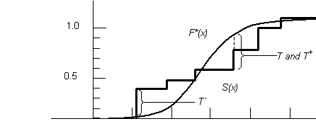
Reject the null hypothesis Ho
at the level of significance a
(meaning the two distributions are not alike) if the appropriate test statistic (T, T+ or
T-) exceeds the 1 - a
quantile (w1 - a)
as given in the Table C-10, otherwise accept Ho (meaning the two distributions are alike). Note
that the two-sided test statistic
T is always equal to the larger of
the one-sided test statistics T+ and
T-.
Conover (1999, p.438-439) details one of the most useful
features of the Kolmogorov two-sided test, the ability to form a confidence
band for the true unknown distribution
function F (x). This allows upper and lower bounds to be
placed on the graph of the EDF S (x)
and make the statement that the unknown distribution function F
(x) lies entirely within those bounds, with 1- a confidence that the statement is
correct. The reader is directed to the
reference for more details and the methodology.
Environment Example:
In a reexamination of previous papers that fitted air quality data to hypothetical probability
distributions (Chock and Sluchak, Atmospheric Environment, V.20, N.5, 1986),
the researchers built the case that the six goodness of fit (GOF) methods used gave varying results as
to which of the six hypothesized parent distributions the samples were drawn
from. Air quality data are frequently fitted to
hypothetical probability distributions--in this case to lognormal, gamma, beta,
Weibull and Johnson distributions--with the intent of using the distributions
to predict the number of days on which observed ozone and carbon monoxide
concentrations exceed National Ambient Air Quality Standards. Since these GOF methods did not agree, and
for other reasons stated by the researchers, they conclude that “best” fitted
distributions of air quality data
should not be used to predict the very extreme values used in setting air
quality standards. They suggest that a
less-extreme standard, such as using the 95th percentile of the data, would
significantly reduce the impact of the intrinsic uncertainty of the
estimate.
Only three of the six GOF methods used are statistical GOF methods capable of
supporting hypothesis testing:
chi-square, Kolmogorov-Smirnov, and Cramer-von Mises-Smirnov. In reporting the results, the significance for the chi-square
GOF test is given. However, for the
other two tests the significances are not reported or is any hypothesis testing done. The researchers only use qualitative
statements such as “fit the . . . data
set well.” It is recommended that when
possible, and it is certainly possible with statistical GOF tests, a hypothesis test be done at a
stated significance level or a p-value be reported to allow the reader to
adequate evaluate the reported results.
While the six GOF tests do vary in selecting the best fitting distribution, it
is interesting to note that the three statistical GOF tests all did yield the
same result. These three
methods--Chi-square, Kolmogorov-Smirnov, and Cramer-von Mises-Smirnov--all
picked the same distribution of
those offered as the best fitting for the two samples. They did, however, pick different
distributions for each of the two samples.
The three other GOF tests employed by the researchers--absolute
deviation, weighted absolute deviation, and log-likelihood value-- gave varying
results.
The two samples used by the researchers to support their arguments were
actually the same data. The first
sample had 122 data points and
the second sample was 120 of
these points, the two removed points being the lowest values, deemed to be
outliers by the authors. The best
fitting hypothetical distributions for the two samples differed. This illustrates the importance of
“outliers.” It is recommended that
“outliers” never be removed from data
without good justification.
Furthermore, that justification should be stated in the findings--as the
authors did in this example paper.
Obviously, the removal of these two “outliers” had a significant impact
on the conclusions drawn in this paper and interested readers would want to
know the reasons for removing the two outliers so they can form their own conclusions.
It should be noted once again the importance of specificity when discussing
statistical tests used to reach conclusions--either by citing a reference for
the statistical test(s) used or by reporting sufficient information such that
the reader can accurately deduce the specific test statistic/method used. In this example the researchers list the
results for the “Kolmogorov-Smirnov statistic” GOF test for each of the six
distributions tested. The values range from about 5.5 to 9.5. The Kolmogorov GOF test described in this
manual uses the maximum “vertical distance” between the empirical distribution function
(EDF) of the data and the cumulative distribution function (CDF) of the hypothesized
distribution as the test statistic.
This means that the test statistic
ranges from 0.0 to 1.0. Obviously the
researchers were using some other form of a Kolmogorov-Smirnov type test statistic and a compatible set
tables to interpret the results. Again,
researchers are cautioned not to use the test statistics given in this manual with tables taken from some
other source unless certain that they are compatible. The researchers did cite a reference for the Cramer-von
Mises-Smirnov GOF test they used. This
test was devised by the three statisticians for whom it is named between 1928
and 1936. The citation given by the
researchers was a 1946 book by Cramer.
While this documents the test adequately, such an old reference may be
generally inaccessible to most readers.
Thought should be given to citing more current references to assist the
interested reader.
The Kolmogorov GOF test assumes the theorized distribution is completely
specified, i.e., no parameters have to be estimated from the sample. If parameters are estimated from the sample,
then it becomes conservative. To
provide more precise tests, additional tables have been developed using the
same Kolmogorov test statistic. The
tables vary for the specific hypothesized distribution being tested.
These tests are still nonparametric because the validity of the test (the a
level) does not depend on untested assumptions regarding the population distribution. Rather, the population distribution form
is the hypothesis being
tested.
Lilliefors developed a GOF test in 1967, which tests the
composite hypothesis of
normality. Under this method, the null hypothesis states that the sample
is drawn, not from a single specified distribution, but from the family of
normal distributions. This allows that
neither the mean nor variance of the normal
distribution must be specified. Conover
(1999, p.443-447) provides the detailed method and table for this test. In a similar manner, Lilliefors later (1969)
developed a GOF test for the family of exponential distributions.
This test method and tables are also detailed in Conover (1999, p.447-449). The power of both these tests are believed to be greater than
the chi-square test. A potentially
useful application of the Lilliefors GOF test for exponential distributions is
when a researcher is theorizing that when events occur randomly, the time
between events follow an exponential
distribution. In this situation, the
test can be used as a test of randomness of the data.
Another test for normality of an EDF is the Shapiro-Wilk
GOF test. Some studies have concluded
that this test has greater power
than the Lilliefors test in many situations.
This test is not of the Kolmogorov-type. Conover (1999, p.450-451) provided the detailed method and tables
for this test. A useful feature of this
test is highlighted though an example by Conover, wherein several independent
goodness-of-fit tests are combined into one overall test of normality. This allows several small samples from
possibly different populations, which by themselves are insufficient to reject
the hypothesis of normality, to
be combined and thereby provide enough evidence to disprove normality.
3) The
samples are random samples.
4) The
two samples are mutually independent.
5) The
measurement scale is at least ordinal.
6) The
theoretical distribution (and by
implication the sample
distribution) is continuous. May still
be used for discrete distributions but doing so leads to a conservative test.
The data
consist of two independent random samples, one of size n, X1, X2, . . . , Xn, associated with some unknown distribution function F (x).
The other sample is of
size m, Y1, Y2, . . . , Ym, associated with
some unknown distribution function
G (x).
A. Two-sided test
Ho: F (x) = G (x) for all x
Ha: F (x) ¹
G (x) for at least one x
B. One-sided test
Ho: F (x) £ G (x) for
all x
Ha: F (x) > G (x) for at least one x
This
is used when the distributions are suspected of being the same except that the sample distribution F (x) is shifted to the left of the sample distribution G (x).
In other words, the X values
of the F (x) tend to be smaller than
the Y values of the G (x).
This is a more general test than testing for the distributions only
differing by a location parameter
(means or medians).
C. One-sided test
Ho: F (x) ³ G (x) for
all x
Ha: F (x) < G (x) for at least one x
This
is the one-side test to use when the distributions are suspected of being the
same except that the sample
distribution F (x) (X values) is (larger) shifted to the
right of the sample
distribution G (x) (Y values).
TEST STATISTIC (T,
T +, T -)
OF SMIRNOV GOF TEST FOR TWO INDEPENDENT SAMPLES
Let S1
(x) be the empirical
distribution function (EDF) based on the random sample X1, X2, . . . , Xn. Let S2x) be the empirical distribution function
(EDF) based on the other random sample Y1,Y2,. . , Ym. The
test statistic T is defined differently for hypotheses
sets A, B and C.
A. Two sided test: The test statistic
T is the maximum difference between
the two EDFs, S1(x) and S2(x):
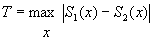
B. One-sided test: The test statistic
T+ is the maximum difference by S1(x) above S2(x):
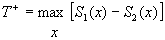
C. One-sided test: The test statistic
T- is the maximum difference by S2(x) above S1(x):
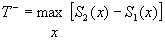
Reject the null hypothesis Ho
at the level of significance a
(meaning the two distributions are not alike) if the appropriate test statistic (T, T+ or
T-) exceeds the 1 - a
quantile (w1 - a)
as given in the Table C-11 of n = m or Table C-12 if n ¹ m, otherwise accept Ho (meaning the two
distributions are alike). Note that the two-sided test statistic T is always equal to the larger of the one-sided test statistics T+ and
T-.
This test is an extension of the two-sided Smirnov test,
which may be used for any number of equal size samples. However, tables for three samples are all
that are readily available in the reference given. Similar to finding the maximum distance between S1 (x) and S2 (x)
for the Smirnov test, the Birnbaum-Hall test find the maximum distance that
exists between any combination of two of the three EDFs being tested: S1 (x), S2 (x), S3 (x).
Conover (1980, p.377-379) details the methodology for this GOF test for Ordinal scale or better data and includes the necessary
table for finding the critical values for three samples. However, Conover omits this test in the
third edition of his book (1999) because most data sets are not of equal size, a requirement of this
test. For multiple samples of unequal
size, the researcher can use the nonparametric Chi-square GOF test for two or
more independent samples.
These tests are similar to the Birnbaum-Hall tests but
tables are available from Conover (1980, p.379-384) for up to 10 samples, which
must all be of the same size. Again
however, Conover (1999) omits these tests in the third edition of his book
(1999) because most data sets
are not of equal size, a requirement of these tests. The Chi-square GOF test for two or more independent samples can
be used when dealing with unequal sample
sizes.